Bayesian regression with multiple data chunks:
In this question, you will generate datasets and calculate posterior distributions. If you have trouble, at least try to work out roughly what should happen for each part.
We will use the probabilistic model for regression models from the lectures: \[\notag p(y\g \bx,\bw) = \N(y;\,f(\bx;\bw),\,\sigma_y^2). \]
In this question, we set \(f(\bx;\bw) = \bw^\top \bx\) and assume a diagonal prior covariance matrix: \[\notag p(\bw) = \N(\bw;\,\bw_0,\,\sigma_{\bw}^2\I). \]
From the lecture notes (w4a), we have for the posterior distribution \(p(\bw\g \D) = \N(\bw;\, \bw_N, V_N)\) with: \[\begin{align} V_N &= \sigma_y^2(\sigma_y^2V_0^{-1} + \Phi^\top \Phi)^{-1},\\ \bw_N &= V_N V_0^{-1}\bw_0 + \frac{1}{\sigma_y^2}V_N \Phi^\top\by. \end{align}\] With \(\Phi=X\) and \(V_0 = \sigma_{\bw}^2\I\), we get: \[\begin{align} V_N &= \sigma_y^2(\sigma_y^2\frac{1}{\sigma_{\bw}^2}\I + X^\top X)^{-1},\\ \bw_N &= V_N\frac{1}{\sigma_{\bw}^2}\I\bw_0 + \frac{1}{\sigma_y^2}V_N X^\top\by. \end{align}\]
What distribution with what parameters is \(p(\bw\g \D)\) approaching when we let \(\sigma_{\bw}^2\) approach infinity? Please justify your answer.
Answer:
In the limit \(\sigma_{\bw}^2 \rightarrow \infty\), we have \(V_N \rightarrow \sigma_y^2 (X^\top X)^{-1}\) and \(\bw_N \rightarrow (X^\top X)^{-1}X^\top\by\), as long as \((X^\top X)^{-1}\) exists. So \(p(\bw\g \D)\) is approaching a Gaussian distribution with mean \((X^\top X)^{-1}X^\top\by\) and covariance matrix \(\sigma_y^2 (X^\top X)^{-1}\).
A connection to the least squares solution: The posterior becomes peaked around \((X^\top X)^{-1}X^\top\by\), which is the least squares weight vector (when there is a unique solution). We derived this expression in note w3b. We can also sketch why this should be the least squares solution: The posterior is Gaussian, so its mean is equal to the mode, or the mode of the log posterior, which up to a constant is the sum of the log likelihood and log prior. As the prior gets broader, and tends to a constant for reasonable weights, we just maximize the log likelihood, which we can do by minimizing the sum of square residuals.
For the rest of the question, we assume \(\bw = [w_1 ~~ w_2]^\top\) and \(\bx = [x_1 ~~ x_2]^\top\), and \(\sigma_y^2 = 1^2 = 1\), and \(\bw_0 = [-5 ~~ 0]^\top\), and \(\sigma_{\bw}^2 = 2^2 = 4\).
Generating data: Below, we provide code for generating some synthetic dataset.
import numpy as np
from numpy.random import randn, uniform
import matplotlib.pyplot as plt

D = 2 # Dimension of the weight space
N_Data_1 = 15 # Number of samples in dataset 1
N_Data_2 = 30 # Number of samples in dataset 2
sigma_w = 2.0
prior_mean = [-5, 0]
prior_precision = np.eye(D) / sigma_w**2
# We summarize distributions using their parameters
prior_par = {'mean': prior_mean, 'precision': prior_precision}
# Here we draw the true underlying w. We do this only once
w_tilde = sigma_w * randn(2) + prior_mean
# Draw the inputs for datasets 1 and 2
X_Data_1 = 0.5 * randn(N_Data_1, D)
X_Data_2 = 0.1 * randn(N_Data_2, D) + 0.5
# Draw the outputs for the datasets
sigma_y = 1.0
y_Data_1 = np.dot(X_Data_1, w_tilde) + sigma_y * randn(N_Data_1)
y_Data_2 = np.dot(X_Data_2, w_tilde) + sigma_y * randn(N_Data_2)
# The complete datasets
Data_1 = {'X': X_Data_1,
          'y': y_Data_1}
Data_2 = {'X': X_Data_2,
          'y': y_Data_2}
Explanation: First, we draw a \(\tilde{\bw}\) from the prior distribution (i.e. draw a sample from the Gaussian). In the whole dataset generation process, we draw this \(\tilde{\bw}\) only once and keep it constant.
We then generate two chunks of data \(\D_1\) and \(\D_2\). For chunk \(\D_1 = \{\bx^{(n)},y^{(n)}\}_{n=1}^{15}\), we generate 15 input-output pairs where each \(\bx^{(n)}\) is drawn from \(\N(\bx^{(n)};\,\mathbf{0},0.5^2\I)\). For chunk \(\D_2 = \{\bx^{(n)},y^{(n)}\}_{n=16}^{45}\), we generate 30 input-output pairs where each \(\bx^{(n)}\) is drawn from \(\N(\bx^{(n)};\,[0.5 ~~ 0.5]^\top,0.1^2\I)\). For both chunks, we draw the \(y^{(n)}\) outputs using the \(p(y\g \bx,\bw)\) observation model above.
We use Python dictionaries to better organise the dataset and parameters: prior_par holds the parameters of the prior distribution and Data_1 and Data_2 hold the two chunks of data \(\D_1\) and \(\D_2\), respectively. If you haven’t worked with dictionaries before, you can think of them as collections of stored variables which can be accessed by specified keys. For instance, you can access X_Data_1 in Data_1 with the expression Data_1['X']. Here, Data_1 is the dictionary, X_Data_1 is the stored variable and X is the key.
Complete the following function for calculating the posterior parameters. To avoid calculating inverse matrices, we keep track of the precision matrices \(K_0 = V_0^{-1}\) and \(K_N = V_N^{-1}\) and use the update equations: \[\begin{align} K_N &= K_0 + \frac{1}{\sigma_y^2}X^\top X,\\ \bw_N &= K_N^{-1} K_0\bw_0 + \frac{1}{\sigma_y^2}K_N^{-1} X^\top\by. \end{align}\]
Answer:
def posterior_par(prior_par, Data, sigma_y):
    """Calculate posterior parameters.

    Calculate posterior mean and covariance for given prior mean and
    covariance in the par dictionary, given data and given noise
    standard deviation.
    """
    X = Data['X']
    y = Data['y']
    var_y = sigma_y**2
    w_0 = prior_par['mean']
    K_0 = prior_par['precision']
    # The next line corresponds to:
    #  V_N = var_y * inv(var_y * V_0_inv + np.matmul(X.T, X))
    K_N = K_0 + np.matmul(X.T, X) / var_y
    # The following lines correspond to:
    #  w_N = np.dot(V_N, np.dot(V_0_inv, w_0))
    if y.size > 0:
        w_N = np.linalg.solve(K_N, np.dot(K_0, w_0) + np.dot(X.T, y) / var_y)
    else:
        w_N = np.linalg.solve(K_N, np.dot(K_0, w_0))
    return {'mean': w_N, 'precision': K_N}
Here, we are calling
np.linalg.solvetwice. A more efficient alternative would exploit that \(K_N\) is positive definite by calculating the Cholesky once and using it twice withscipy.linalg.cho_solve.Write a function that takes a mean and a covariance of any 2D multivariate Gaussian as input arguments. The function should then visualize the Gaussian by drawing 400 samples from the distribution and showing the samples in a 2D scatter plot. Let the function also show the mean as a bold cross in the same plot. To implement this function, you can use the
choleskyandsolve_triangularfunctions fromscipy.linalg. Then visualise the prior distribution and discuss the relationship between the parameters and the belief expressed by the prior.
Answer:
import scipy.linalg as sla

def visualise_par(par, label, colour):
    ''' Visualises a multivariate normal distribution with given mean and
        covariance matrix in the par dictionary.
    '''
    D = len(par['mean'])
    # The next three lines correspond to:
    #  samples = multivariate_normal(par['mean'],
    #                                inv(par['precision']), 400)
    L = sla.cholesky(par['precision'], lower=True)
    samples = sla.solve_triangular(L, randn(D, 400), trans=1,
                                   lower=True).T + par['mean']
    plt.scatter(samples[:, 0], samples[:, 1], s=1, label=label, c=colour)
    plt.plot(par['mean'][0], par['mean'][1], marker='X', c='k')
    plt.xlim([-10,0])
    plt.ylim([-5,5])
    plt.xlabel('$w_1$')
    plt.ylabel('$w_2$')

plt.figure(1)
plt.clf()
visualise_par(prior_par,
              label='$p(\mathbf{w})$',
              colour='b')
plt.legend()
plt.show()
There will be variability in the plots you generate, in particular regarding the location of \(\tilde{\bw}\), but the plot should look similar to the following:
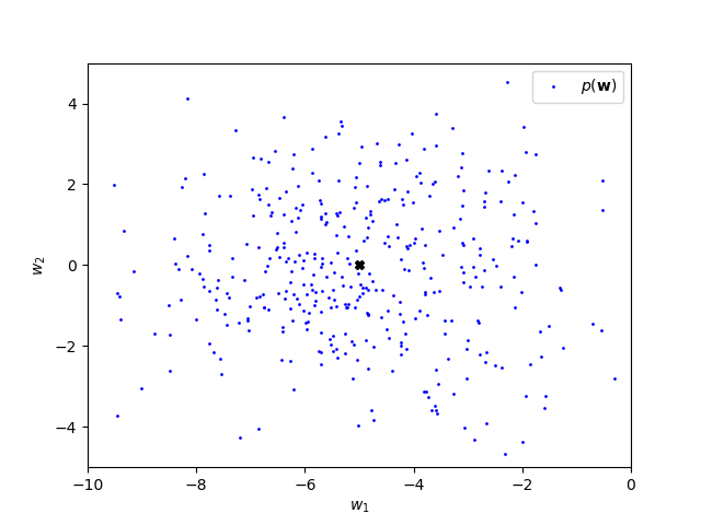
The prior mean can be interpreted as a belief that \(w_1\) is probably negative (and around -5) while \(w_2\) being negative is just as plausible as \(w_2\) being positive. The standard deviation is the same for \(w_1\) and \(w_2\) meaning that we are just as certain about \(w_1\) being close to \(-5\) as we are about \(w_2\) being close to 0. Moreover, the correlation is zero, meaning that we don’t believe in any relationship between \(w_1\) and \(w_2\).
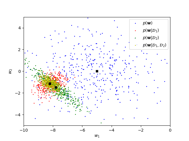
Using the functions from question parts b) and c), calculate and visualise the posterior distributions that you get after observing:
- dataset \(\D_1\), i.e. \(p(\bw\g \D_1)\)
- dataset \(\D_2\) but not \(\D_1\), i.e. \(p(\bw\g \D_2)\)
- datasets \(\D_1\) and \(\D_2\), i.e. \(p(\bw\g \D_1,\D_2)\)
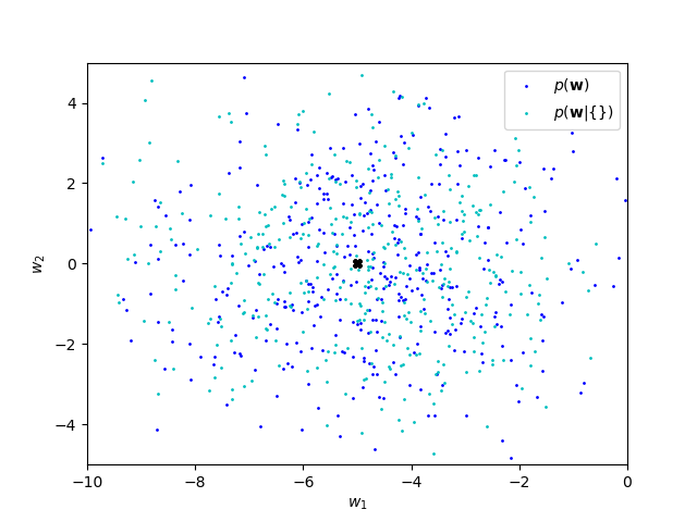
- no observations, i.e. \(p(\bw\g \{\})\)
Answer:
Here see that the two data chunks constrain the broad prior distribution (no observations) in different ways. Conditioning on both datasets incorporates the constraints from both chunks.
# We combine datasets 1 and 2 by stacking the matrices / vectors
Data_1_2 = {'X': np.vstack((X_Data_1, X_Data_2)),
            'y': np.concatenate((y_Data_1, y_Data_2))}
# Calculate posterior parameters
posterior_par_1 = posterior_par(prior_par, Data_1, sigma_y)
posterior_par_2 = posterior_par(prior_par, Data_2, sigma_y)
posterior_par_1_2 = posterior_par(prior_par, Data_1_2, sigma_y)
# Visualise prior and posterior distributions
plt.figure(2)
plt.clf()
visualise_par(prior_par,
              label='$p(\mathbf{w})$',
              colour='b')
visualise_par(posterior_par_1,
              label='$p(\mathbf{w}|\mathcal{D}_1)$',
              colour='r')
visualise_par(posterior_par_2,
              label='$p(\mathbf{w}|\mathcal{D}_2)$',
              colour='g')
visualise_par(posterior_par_1_2,
              label='$p(\mathbf{w}|\mathcal{D}_1,\mathcal{D}_2)$',
              colour='y')
plt.legend()
plt.show()
# Here we construct an empty dataset
Data_nodat = {'X': np.empty([0, D]),
              'y': np.empty([0, 1])}
# The posterior for an empty dataset will be the prior
plt.figure(3)
plt.clf()
posterior_par_nodat = posterior_par(prior_par, Data_nodat, sigma_y)
visualise_par(prior_par,
              label='$p(\mathbf{w})$',
              colour='b')
visualise_par(posterior_par_nodat,
              label='$p(\mathbf{w}|\{\})$',
              colour='c')
plt.legend()
plt.show()
With more data, the posterior should become sharper with a mean closer to \(\tilde{\bw}\):
With no observed data, the posterior corresponds to the prior:
- Take the posterior that you got in d) for \(p(\bw\g \D_1)\) and now use it as a prior. Calculate the new posterior that you get after observing \(\D_2\). Numerically compare the mean and covariance with those of \(p(\bw\g \D_1,\D_2)\).
Answer:
We should find that it doesn’t matter if we update our beliefs in two chunks, or all at once. Our beliefs should be the same given both datasets regardless of how we compute them.
We use the \(\bw_N\) and the \(K_N\) that we got for \(p(\bw\g \D_1)\) and use them as our new \(\bw_0\) and \(K_0\) in the equations from part b): \[\begin{align} K_N &= K_0 + \frac{1}{\sigma_y^2}X^\top X,\\ \bw_N &= K_N^{-1} K_0\bw_0 + \frac{1}{\sigma_y^2}K_N^{-1} X^\top\by. \end{align}\]
# Update the posterior that we got for Data_1 with Data_2
posterior_par_c = posterior_par(posterior_par_1, Data_2, sigma_y)
# The posterior is the same as the one we got in b)
plt.figure(4)
plt.clf()
visualise_par(prior_par,
              label='$p(\mathbf{w})$',
              colour='b')
visualise_par(posterior_par_1_2,
              label='$p(\mathbf{w}|\mathcal{D}_1,\mathcal{D}_2)$',
              colour='y')
visualise_par(posterior_par_c,
              label='Posterior update',
              colour='m')
plt.legend()
plt.show()
print('p(w|D_1,D_2):')
print(posterior_par_1_2)
print('Posterior update:')
print(posterior_par_c)
The posteriors should be identical. While the samples will be different, the point clouds should be on top of each other:
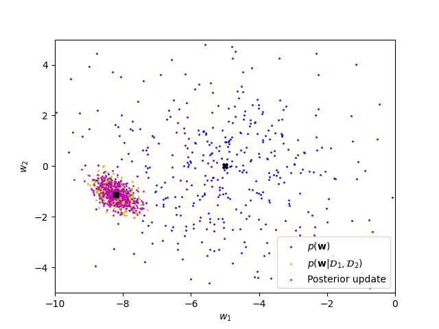
The numerical means and covariance / precision matrices should match (almost) perfectly.
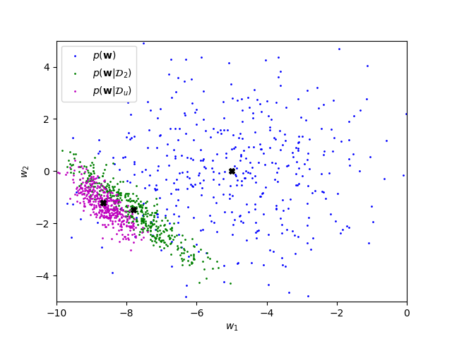
- Is it important that the inputs were drawn from Gaussian distributions? What would happen if the \(\bx^{(n)}\) in \(\D_2\) were drawn from a uniform distribution on the unit square?
Answer:
In our formalism, we don’t make use of any distribution of the input. So with the uniform distribution, we can still apply the same equations from the lecture notes.
# For dataset 2, draw uniform samples instead of Gaussian samples
X_Data_u = uniform(size=D*N_Data_2).reshape([N_Data_2, D])
# Draw the corresponding outputs
y_Data_u = np.dot(X_Data_u, w_tilde) + sigma_y * randn(N_Data_2)
Data_u = {'X': X_Data_u,
          'y': y_Data_u}
# Calculate the posterior for the new dataset
posterior_par_u = posterior_par(prior_par, Data_u, sigma_y)
# Compare to the posterior that we originally got for dataset 2
plt.figure(5)
plt.clf()
visualise_par(prior_par, label='$p(\mathbf{w})$', colour='b')
visualise_par(posterior_par_2,
              label='$p(\mathbf{w}|\mathcal{D}_2)$',
              colour='g')
visualise_par(posterior_par_u,
              label='$p(\mathbf{w}|\mathcal{D}_u)$',
              colour='m')
plt.legend()
plt.show()
The data sampled from the uniform distribution will generally lead to a sharper posterior distribution. This is because the Gaussian that we used to generate \(\D_2\) forms a sharp blob around \([0.5, 0.5]^\top\), while the uniform distribution is more spread out with the same mean. Thus, the diagonal elements of \(X^\top X\) will on average be greater when sampling from the uniform distribution rather than the Gaussian: \[\E[X_kX_k] = \sigma^2 + \E[X_k]^2,\] where \(\sigma^2\) is the variance of the distribution sampled from (you get this equation from rearranging the equation for the variance). \(\E[X_k]\) is the same for both distributions, but the variance of the uniform distribution is \(\frac{1}{12}\) while the variance of the Gaussian is \(0.01\). As can be seen in the equation for \[V_N^{-1} = V_0^{-1} + \frac{1}{\sigma_y^2}X^\top X,\] this results in higher precision and lower covariance:
- Now assume that our observations \(y\) are corrupted by additional Gaussian noise: \[\notag p(z\g \bx,\bw) = \N(z;\, y,\sigma_z^2). \] So we now observe datasets \(\D_z = \{\bx^{(n)},z^{(n)}\}_{n=1}^{N}\). What is the new posterior distribution \(p(\bw \g \D_z)\)? Hint: Recall how you did Question 1.a) of this sheet.
Answer:
We have \[ p(y\g \bx,\bw) = \N(y;\,f(\bx;\bw),\,\sigma_y^2), \] or put differently, \[ y = f(\bx;\bw) + \nu_y, \] where \(\nu_y \sim \N(0, \sigma_y^2)\). With \(p(z\g \bx,\bw) = \N(z;\, y,\sigma_z^2)\), we also have \[ z = y + \nu_z = f(\bx;\bw) + \nu_y + \nu_z, \] where \(\nu_z \sim \N(0, \sigma_z^2)\). Recall from Question 1.a) that sums of independent Gaussian random variables are again Gaussian distributed, with its mean being the sum of the two means and its variance being the sum of the two variances. Thus, we can express \(z\) as \(z = f(\bx;\bw) + \nu_{y,z}\) where \(\nu_{y,z} \sim \N(0, \sigma_y^2 + \sigma_z^2)\). So, all we have to do is to replace \(\sigma_y^2\) with \(\sigma_y^2 + \sigma_z^2\) in the posterior distribution and get \(p(\bw\g \D_z) = \N(\bw;\, \bw_N, V_N)\), where \[\begin{align} V_N &= (\sigma_y^2+\sigma_z^2)((\sigma_y^2+\sigma_z^2)\frac{1}{\sigma_{\bw}^2}\I + X^\top X)^{-1},\\ \bw_N &= V_N\frac{1}{\sigma_{\bw}^2}\I\bw_0 + \frac{1}{\sigma_y^2+\sigma_z^2}V_N X^\top\bz. \end{align}\]
Notes:
For generating the data, we have drawn a \(\bw\) from the same prior distribution that we used for calculating the posteriors. In real applications, the prior distribution expresses beliefs (which could be misguided) about an unknown constant, or is chosen for mathematical convenience. An informative prior could reduce the amount of data we need to observe, but an overly-confident prior could give us an overly-confident posterior.
More practice with Gaussians:
\(N\) noisy independent observations are made of an unknown scalar quantity \(m\): \[\notag x\nth \sim \N(m, \sigma^2). \]
- We don’t give you the raw data, \(\{x\nth\}\), but tell you the mean of the observations: \[\notag \bar{x} = \frac{1}{N} \sum_{n=1}^N x\nth. \] What is the likelihood1 of \(m\) given only this mean \(\bar{x}\)? That is, what is \(p(\bar{x}\g m)\)?2
Answer:
The mean of some Gaussian outcomes, like any linear combination, is Gaussian distributed. So we just have to identify the mean and variance of this derived quantity. The mean: \[ \E[\bar{x}] = \frac{1}{N} \sum_{n=1}^N \E[x\nth] = \frac{1}{N} \sum_{n=1}^N m = m. \] The variance: \[\begin{align} \text{var}[\bar{x}] &= \frac{1}{N^2} \text{var}\left[\sum_{n=1}^N x\nth\right] &= \frac{1}{N^2} \left[N \sigma^2\right] = \frac{\sigma^2}{N}. \end{align}\] where variances add because the noisy outcomes are independent. So: \[ p(\bar{x}\g m) = \N(\bar{x};\, m,\, \sigma^2/N). \]
A sufficient statistic is a summary of some data that contains all of the information about a parameter.
Show that \(\bar{x}\) is a sufficient statistic of the observations for \(m\), assuming we know the noise variance \(\sigma^2\). That is, show that \(p(m\g \bar{x}) \te p(m\g \{x\nth\}_{n=1}^N)\).
If we don’t know the noise variance \(\sigma^2\) or the mean, is \(\bar{x}\) still a sufficient statistic in the sense that \(p(m\g \bar{x}) \te p(m\g \{x\nth\}_{n=1}^N)\)? Explain your reasoning.
Note: In i) we were implicitly conditioning on \(\sigma^2\): \(p(m\g \bar{x}) = p(m\g \bar{x}, \sigma^2)\). In this part, \(\sigma^2\) is unknown, so \(p(m\g \bar{x}) = \int p(m,\sigma^2\g \bar{x})\,\mathrm{d}\sigma^2\). Although no detailed mathematical manipulation (or solving of integrals) is required.
Answer:
The posterior given the observations comes from Bayes’ rule: \[\begin{align} p(m\g \{x\nth\}_{n=1}^N) &\propto p(m)\,p(\{x\nth\}_{n=1}^N\g m) \\[1ex] &\propto p(m)\prod_n \N(x\nth;\, m,\, \sigma^2)\\ &\propto p(m)\, \exp\!\left(-\frac{1}{2\sigma^2}\sum_n (x\nth-m)^2\right)\\ &\propto p(m)\, \exp\!\left(-\frac{Nm^2}{2\sigma^2} + \frac{m \sum_n x\nth}{\sigma^2}\right). \end{align}\] The proportionality sign, ‘\(\propto\)’, means that we can drop any multiplicative term that doesn’t depend on \(m\).
Given just the mean \(\bar{x}\) the posterior would be: \[\begin{align} p(m\g \bar{x}) &\propto p(m)\,p(\bar{x}\g m) \\ &\propto p(m) \,\N(\bar{x};\, m,\, \sigma^2/N)\\ &\propto p(m)\, \exp\!\left(-\frac{N}{2\sigma^2} (\bar{x}-m)^2\right)\\ &\propto p(m)\, \exp\!\left(-\frac{Nm^2}{2\sigma^2} + \frac{m N\bar{x}}{\sigma^2}\right), \end{align}\] which, substituting the definition of \(\bar{x}\), is equal to the posterior given all of the observations. Therefore \(\bar{x}\) is a sufficient statistic. Our beliefs about the parameter \(m\) given just \(\bar{x}\) are identical to those given the whole dataset.
The working above assumed that we knew the variance \(\sigma^2\). If we don’t know \(\sigma^2\) then \(\bar{x}\) is not sufficient for computing the posterior over the mean. Counter example: if all the \(x\nth\) samples were identical, then we would infer that the variance is zero and have a delta-function posterior over the mean. If the \(x\nth\) samples had high variance (which they could have with the same mean \(\bar{x}\)), we’d realize the variance is larger, and not be certain about the mean. We can still use \(\bar{x}\) as a point-estimate of the mean, it just doesn’t tell us the whole posterior distribution.
Purpose of Q2:
Computing the posterior in Bayesian linear regression is just an example of dealing with noisy observations of linear combinations of Gaussian variables. We encounter similar examples when computing predictions in Bayesian linear regression and Gaussian processes. We can do a lot of useful statistical reasoning if we know how to deal with Gaussians, so it’s worth practicing manipulating them. This question was meant to contain some easier manipulations than some of the ones we’ve seen in lectures.
Much of machine learning is about compressing some useful knowledge from a large dataset into a learned model. The notion of a sufficient statistic is sometimes useful: it tells us some narrow situations in which we can replace a large dataset with some statistics without losing anything.
Bonus question: Conjugate priors (This question sets up some intuitions about the larger picture for Bayesian methods.)
A conjugate prior for a likelihood function is a prior where the posterior is a distribution in the same family as the prior. For example, a Gaussian prior on the mean of a Gaussian distribution is conjugate to Gaussian observations of that mean.
The inverse-gamma distribution is a distribution over positive numbers. It’s often used to put a prior on the variance of a Gaussian distribution, because it’s a conjugate prior.
The inverse-gamma distribution has pdf (as cribbed from Wikipedia): \[ p(z\g \alpha, \beta) = \frac{\beta^{\alpha}}{\Gamma(\alpha)}\, z^{-\alpha-1}\, \exp\!\left(-{\frac{\beta}{z}}\right), \qquad \text{with}~\alpha>0,~~\beta>0, \] where \(\Gamma(\cdot)\) is a gamma function.3
Assume we obtain \(N\) observations from a zero-mean Gaussian with unknown variance, \[ x\nth \sim \N(0,\, \sigma^2), \quad n = 1\dots N, \] and that we place an inverse-gamma prior with parameters \(\alpha\) and \(\beta\) on the variance. Show that the posterior over the variance is inverse-gamma, and find its parameters.
Hint: you can assume that the posterior distribution is a distribution; it normalizes to one. You don’t need to keep track of normalization constants, or do any integration. Simply show that the posterior matches the functional form of the inverse-gamma, and then you know the normalization (if you need it) by comparison to the pdf given.
Answer:
The posterior is given by Bayes’ rule. I’m going to write the variance as \(v\te\sigma^2\) so the square won’t confuse me when comparing coefficients. \[\begin{align} p(v\g \{x\nth\},\alpha,\beta) &\propto v^{-\alpha-1} \exp\!\left(-{\frac{\beta}{v}}\right) \prod_n \N(x\nth;\, 0,\, v)\\ &\propto v^{-\alpha-1} \exp\!\left(-{\frac{\beta}{v}}\right) v^{-N/2} \exp\!\left(-\frac{1}{2v}\sum_n(x\nth)^2\right)\\ &\propto v^{-(\alpha+N/2)-1} \exp\!\left(-{\frac{\beta+\frac{1}{2}\sum_n(x\nth)^2}{v}}\right)\\ &=\text{inverse-gamma}\!\left[v;\; \alpha+N/2,\; \beta+\frac{1}{2}\sum_n(x\nth)^2\right]. \end{align}\] The posterior is also inverse-gamma, so the prior is conjugate to the likelihood.
Some people aren’t happy with the step to the final line. The distribution has only been written down up to a constant. But that constant is specified: we know the distribution must integrate to one. Therefore the pdf can only be one function, and that function matches the standard form of the inverse-gamma distribution.
Warning: some books and library routines parameterize distributions differently, so you have to be sure that \(\alpha\) and \(\beta\) mean what you think they do before using them with someone else’s result or function.
If a conjugate prior exists, then the data can be replaced with sufficient statistics. Can you explain why?
Answer:
When we have a conjugate prior, it means that the posterior, like the prior, can be expressed as some neat standard distribution. The parameters of that distribution are enough to represent all of our beliefs about the parameters given the data. Therefore these parameters are sufficient statistics: given them, we don’t need to store the data any more.
For completeness, the parameters of the conjugate posterior distribution are sufficient statistics, even if you don’t want to use that conjugate prior. Notation: parameters \(\theta\), data \(\D\), assumption that we should use a conjugate prior \(\C\), and assumption we should use another prior \(\M\). The posterior given a conjugate prior, \[ p(\theta\g \D, \C) = \frac{p(\D\g \theta)\,p(\theta\g \C)}{p(\D\g \C)}, \] is available in a compact form. The posterior given another prior is: \[ p(\theta\g \D, \M) \propto p(\D\g \theta)\,p(\theta\g \M) \propto \frac{p(\theta\g \D, \C)}{p(\theta\g \C)}\,p(\theta\g \M), \] So the parameters of the conjugate prior and posterior distributions summarize everything we need to know about the data to construct beliefs about the parameters. (As long as we haven’t divided by zero. The conjugate prior \(p(\theta\g \C)\) better have full support over the parameters.)
Lessons from Q3:
When we fit parametric models we use the data to set some parameters, and then throw the data away at test time. In the Bayesian approach to prediction, the posterior distribution is the summary of what we have learned from the data. The posterior is only simple to represent (exactly) for conjugate models. In this course we mainly focus on Gaussian models, but there are some other convenient conjugate distributions.