Training, Testing, and Evaluating Different Models

You now have enough knowledge to be dangerous. You could read some data into matrices/arrays in a language like Matlab or Python, and attempt to fit a variety of linear regression models. They may not be sensible models, and so the results may not mean very much, but you can do it.

You could also use more sophisticated and polished methods baked into existing software. Many Kaggle competitions are won using easy-to-use and fast gradient boosting methods (such as XGBoost, LightGBM, or CatBoost), or for image data using ‘convolutional neural nets’, which you can fit with several packages, for example Keras.

How do you decide which method(s) to use, and work out what you can conclude from the results?

1 Baselines

It is almost always a good idea to find the simplest possible algorithm that could possibly give an answer to your problem, and run it. In a regression task, you could report the mean square error of a constant function, \(f(x)\te b\). If you’re not beating that model on your training data, there is probably a bug in your code. If a fancy method does not generalize to new data as well as the baseline, then maybe the problem is simply too hard… or there are more subtle bugs in your code.

It is also usual to implement stronger baselines. For example, why use a neural network if straight-forward linear regression works better? If you are proposing a new method for an established task, you should try to compare to the existing state-of-the art if possible. (If a paper does not contain enough detail to be reproducible, and does not come with code, they may not deserve comparison.)

I’ve heard the following piece of advice for finding a machine learning algorithm to solve a practical problem¹:

“Find a recent paper at a top machine learning conference, like NeurIPS or ICML that’s on the sort of task you need to solve. Look at the baseline that they compare their method to… and implement that.”

If they used a method for comparison, it should be somewhat sensible, but it’s probably a lot simpler and tested than the new method. And for many applications, you won’t actually need this year’s advance to achieve what you need.

2 Training and Test Sets and Generalization Error

Video: Generalization Error and Monte Carlo (13 minutes)
Generalization error is the expected loss on a random future example. We estimate it using a held-out test set, which is an example of a “Monte Carlo” estimate, or statistical sampling to estimate a large integral or sum.

We may wish to compare a linear regression model, \(f(\bx;\bw,b)=\bw^\top\bx + b\), to a constant function baseline \(f(\bx;b)=b\). The linear regression model can never be beaten on the training data by the baseline, even if the data are random noise. The models are nested: linear regression can become the simpler model by setting \(\bw\te\mathbf{0}\), and obtain the same performance. Then there will almost always be some way to set \(\bw\!\ne\!\mathbf{0}\) to improve the square error slightly.

Thus we cannot use the performance on a training set to pick amongst models. The most complicated model will usually win, and it will always win if the models are nested. Yet in the previous note we saw how dramatically bad the fit can be from models with many parameters.

Instead, we could compare our model to a baseline on new data that wasn’t used when fitting or training the model. This held-out data is usually called a test set. The test set is used to report the error that the model achieves when generalizing to new data, and should only be used for that purpose.

Formally, the generalization error, is the average error or loss that the model function \(f\) would achieve on future test cases coming from some distribution \(p(\bx,y)\): \[ \text{Generalization error} = \E_{p(\bx,y)}[L(y, f(\bx))] = \int L(y, f(\bx))\,p(\bx,y)\intd\bx\intd y, \] where \(L(y, f(\bx))\) is the error we record if we predict \(f(\bx)\) but the output was actually \(y\). For example, if we care about square error, then \(L(y, f(\bx)) = (y\tm f(\bx))^2\).

We don’t have access to the distribution of data examples \(p(\bx,y)\). If we did, we wouldn’t need to do learning! However, we might assume that our test set contains \(M\) samples from this distribution. (That’s a big assumption, which is usually wrong, because the world will change, and future examples will come from a different distribution.) Given this assumption, an empirical (observed) average can be used as what’s called a Monte Carlo estimate of the formal average in the integral above: \[ \text{Average test error} = \frac{1}{M} \sum_{m=1}^M L(y^{(m)}, f(\bx^{(m)})), \qquad \bx^{(m)},y^{(m)}\sim p(\bx,y). \] If the test items really are drawn from the distribution that we are interested in, the expected value of the test error is equal to the generalization error. (Check you can see why.) That means it’s what’s called an unbiased estimate: sometimes it’s too big, sometimes to small, but on average our estimate is correct.

3 Validation or Development sets

Video: Selecting model choices with a validation set (10 minutes)
We choose the order of a polynomial by picking the model that performans best on a held-out validation set. We sketch the same idea for selecting regularization constants, and note that the gap between training and validation performance is not how to select models.

Video: Training, validation, and test sets (9 minutes)
A discussion of why we usually need at least three separate datasets. A training set to fit models; a validation/development set to evaluate different models during developing; and a test set for final evaluation.

We often have many different models that we could consider fitting, and would like to use the one that generalizes the best. These models are often variants of the same model, but with different choices or “hyperparameters”. For example, we can construct different linear regression models by specifying different basis functions (the \(\bphi\) function) and regularization constants \(\lambda\).

We shouldn’t evaluate all of these alternative models on the test set. Selecting a model from many variants often picks a model that did well by chance, and its performance on future data is often lower than on the data used to make the choice. For example, if we test a set of models with different regularization constants \(\lambda\) and select the model with the best test performance, we have fitted the parameter \(\lambda\) to the test set. However, the test set is meant for evaluation, and should be held-out from all procedures that make choices about a model.

Instead we should split the data that’s not held out for testing into a training set and a validation set. We fit the main parameters of a model, such as the weights of a regression model, on the training set. Different variants of the model, perhaps with different regularization parameters, are then evaluated on the validation set to see which settings seem to generalize best. Finally, to report how well the selected model is likely to do on future data, it is evaluated on the test set. We should not evaluate many alternatives on the test set.

Example: the plot below shows some polynomial fits to some training data (blue crosses) with different degrees \(p\). The quadratic curve (\(p\te2\)) is underfitting, and the 9th order polynomial is showing clear signs of overfitting.

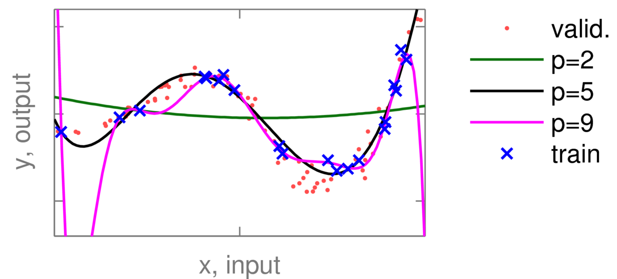
The red dots are validation data: held out points that weren’t used to fit the curves. Training and validation errors were then plotted for polynomials of different orders:

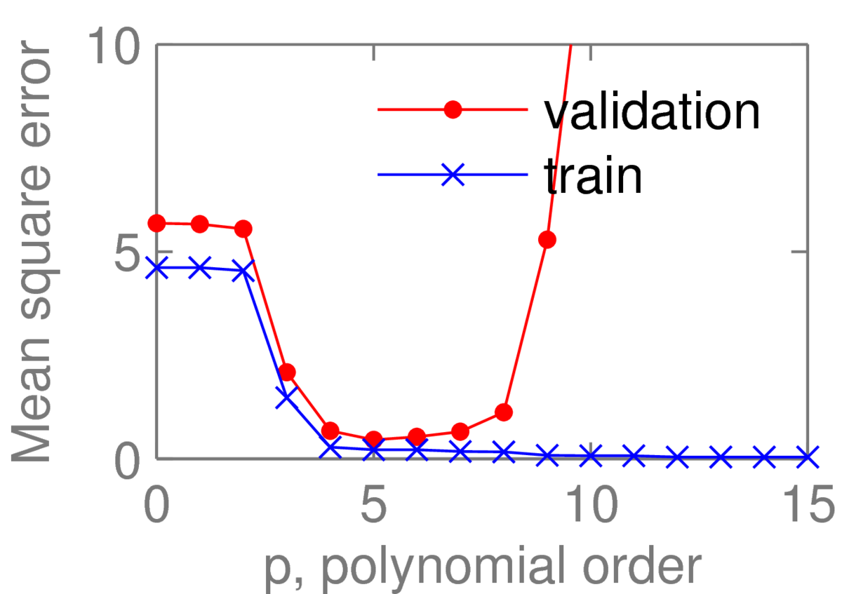
As expected for nested models, the training error falls monotonically as we increase the complexity of the model. However, the fifth order polynomial has the lowest validation error, so we would normally pick that model. Looking at the validation curve, the average error of the fourth to seventh order polynomials all seem similar. If choosing a model by hand, I might instead pick the simpler fourth order polynomial.

4 What to report

After choosing our final model, we evaluate and report its test error. We would normally also report the test error on a small number of reference models to put this number in context: often a simple baseline of our own, and/or a previously-reported state-of-the-art result. We don’t evaluate other intermediate models (with different model sizes or regularization constants) on the test set!

It is often also useful to report training and validation losses, which we can safely report for more models. Researchers following your work can then compare to your intermediate results during their development. If you only give them a test performance, other researchers will be tempted to consult the test performance of their own systems early and often during development.

It can also be useful to look at the training and validation losses during your own model development. If they’re similar, you might be underfitting, and you could consider more complicated models. If the training score is good, but the validation score is poor, that could be a sign of overfitting, so you could try regularizing your model more.

We usually report the average loss on each of the training, validation and test sets, rather than the sum of losses. An average is usually more interpretable as the ‘typical’ loss encountered per example. It is also easier to compare training and validation performance using average errors: because the sets have different sizes, we wouldn’t expect the sum of losses to be comparable.

The validation and test errors, as estimates of generalization error, shouldn’t include a regularization term (such as \(\lambda\bw^\top\bw\), see previous note). Therefore, for comparison, “training error” usually shouldn’t include a regularization term either, even if the cost function being optimized does. On the other hand, there are times when it makes sense to report regularized costs, such as when monitoring convergence during model fitting (in methods we’ll consider later), or checking that nested models have the expected ordering of training costs.

5 Some detail on splitting up the data

How should we split up our data into the different sets? You might see papers that use (for example) 80% of data for training, 10% for validation, and 10% for testing. There’s no real justification for using any fixed set of percentages, but it’s likely that no one would question such a split. What we really want to do is use as much data for training as possible, so that we can fit a good model.² We are limited by the need to leave enough data for validation and testing to choose models and report model performance. Deciding if we have enough validation/test data would require inspecting “error bars” on our estimates, which we’ll cover in a later note.

Given that we want to use as much data for training as possible, we could consider combining our training and validation sets after making model choices (basis functions, regularization constants, etc.) and refit. I’d probably try that sort of trick if trying to win a competition, but usually avoid retraining on validation data in my research. Reason 1: If comparing to other work that uses a particular train/validation split, I try to follow their protocols. I don’t want to just get good numbers: I want a controlled comparison between models, so I can show that my numbers are better because of interesting differences between models. If I’m the first to work on a dataset, I also don’t want to create complicated, expensive protocols for others to follow. Reason 2: for models like neural nets, where an optimizer can find parameters in different regions on every run, I might be unlucky when refitting and fit a worse model. If I don’t have any held out data, I won’t notice.

6 \(K\)-fold cross-validation

A more elaborate procedure called \(K\)-fold cross-validation is appropriate for small datasets, where holding out enough validation data to select model choices leaves too little data for training a good model. The data that we can fit to is split into \(K\) parts. Each model is fitted \(K\) times, each with a different part used as a validation set, and the remaining \(K\tm1\) parts used for training. We select the model choices with the lowest validation error, when averaged over the \(K\) folds. If we want a model for prediction, we then might refit a model with those choices using all the data.

Making statistically rigorous statements based on \(K\)-fold cross-validation performance is difficult. (Beyond this course, and I believe an open research area.)

If there’s a really small dataset, a paper might report a \(K\)-fold score in place of a test set error. In your first project in machine learning, I would try to avoid following such work. To see some of the difficulties, imagine I want to report how good a model class is (e.g., a neural network) compared to a baseline (e.g., linear regression) for some task. But the data I have to do the comparison is small, so I report an average test performance across \(K\)-folds, each containing a training and test set.

What do I do within each fold? Assume I need to make a model choice or choose a “hyperparameter” for each model class, such as the \(L_2\) regularization constant \(\lambda\). As we have already seen, we can’t fit such choices to the training data. But fitting them to the test data would be cheating. I could split off a validation set from the training data. But the dataset is small, so the validation scores would be noisy. So maybe I run \(K\)-fold cross-validation to pick the regularization constant.

The above paragraph was talking about being within a particular fold, so I’ll have to do the \(K\)-fold cross-validation to pick the regularizer \(\lambda\) for each of the outer-loop folds that I’m doing to report test performance.

If you’re not quite following, the take-away message from this part is that doing \(K\)-fold cross-validation carefully can be a confusing and costly mess! While it’s useful for small datasets, I’d try to avoid it in your first machine learning projects, by finding a problem with lots of data. Or try to use methods (like the Bayesian methods covered later in the course) that can deal with hyperparameters without the need for separate validation sets. If you do need to understand the ideas in this section better, you could search for “nested \(K\)-fold cross-validation”.

7 Not fitting the validation and test sets

In the simplest “textbook” prediction setting, we fit a function \(f(\bx; \bw)\) to the training set only. We should then be able to apply that function to individual inputs \(\bx\) in future, giving predictions. In this setting, your code shouldn’t gather any statistics across the whole validation or test set before making predictions. For example it’s common to center data, by subtracting the mean training input from every input. You can view this shift as part of the function, so if you want to apply the function consistently, you should apply the same shift in future (don’t use the mean of the validation or test inputs).

There are settings beyond this course (like “transductive learning”) that look at the validation/test inputs, and it is sometimes a good idea if you know what you are doing. However, your experiments will be simpler if you don’t use any aspect of the validation or test sets to define your function, and it will be easier to interpret your results.

Under no circumstances should your prediction code see the test labels!

7.1 Warning: Don’t fool yourself (or make a fool of yourself)

It is surprisingly easy to accidentally overfit a model to the available test data, and then generalize poorly on future data. For example, someone may have followed good practice for all of their analysis, but then the final test score is disappointing. They then realize that there was something they should probably have done differently, so they change that and try again. Then they have another realization, but after that change the test score gets worse, so they revert that change… and so on.

Each minor re-run of a method, or peek at the test set, doesn’t seem like it could cause any problems individually. But the effects build up. These problems with accidental overfitting are frequently seen on Kaggle. Their competitions display a public leaderboard, based on a test set, but the final rankings are based on a second test set. It is common for some competitors to fall many places when the leaderboard is re-ranked. One such competitor (Greg Park) wrote a reflective blog post on how they had fooled themselves. Despite knowing about cross-validation and the dangers of overfitting, they slowly but surely slipped into fitting the test set. They reached second place on the public leaderboard, but fell dramatically when it was re-ranked… embarrassingly beneath one of the available baselines.

Training on the test set is one of the worst mistakes you can make in machine learning. At best, the results you present will be misleading, and at worst they will be meaningless. Markers of dissertation projects are likely to penalize such poor practice severely. In your own projects, if you can³, I suggest holding out some data that you never look at during the bulk of your research. Pretend it doesn’t exist. Then right at the end, test only the most-interesting models on the totally-held out test set.

8 Limitations of test set errors

Tests on held-out data provide straightforward quantitative comparisons between models. Based on these comparisons, if done properly, we can be fairly sure how well a model will generalize to data drawn from the same distribution.

Future data usually won’t be drawn from the same distribution however. The properties of most systems drift over time. Dealing with these changes is hard, and often ignored. If your data is explicitly provided as a time-series, it’s usual to select a validation set after all of your training data and a test set after that. It’s accepted that test performance is likely to be worse than the validation performance, which will give some estimate of how badly and quickly a system degrades over time. You could also consider online prediction. Rather than having separate training and testing phases, you deal with the data in a stream, predicting each item one at a time in sequence, updating the model with each item after you have predicted it.

Even for stable systems, test set errors only say how well, under the given distribution, the models make predictions. A model with low test error does not necessarily reflect the structure of the real system, and as a result may generalize poorly if used in other ways. For example, you should be careful about attempting to interpret meaning behind the weights in a model. Statistics books are full of examples of how various problems (e.g., selection effects, confounds, and model mismatch) can make you reach completely wrong conclusions about a system from a model’s fitted parameters.⁴

9 Check your understanding

• You should check that you actually followed the details in this note. Could you produce figures like the two illustrating polynomial fits? If not, what do you need to know?

  Could you follow the same idea to pick a \(L_2\) regularizing constant when (for example) fitting a regression problem with a fixed set of RBF basis functions?

  Later in the course, or your career, you might have to explain such a procedure in English, or pseudo-code. And then you might need to implement it.

• Could you adapt your procedure to fit both a regularizing constant, and a width \(h\) shared by a set of RBF basis functions?

  What difficulties do you face as the number of “hyperparameters” (parameters that control the complexity or structure of your model) that you want to set grows?

  Would you have additional difficulties setting separate centres and/or widths for every RBF (not just because it’s a large number of hyperparameters?)?

10 Further Reading

Bishop’s book Sections 1.1 and 1.3 summarize much of what we’ve done so far.

The following two book sections contain more (optional) details. These sections may assume some knowledge we haven’t covered yet.

• Barber’s book covers validation and testing in Sections 13.2.1–2.
• Murphy’s book Section 7.5, p225, discusses Ridge regression (L2 regularization) and Fig 7.8a shows training and test (should be validation) curves for different regularization constants.

Keen students could read the following book chapter by Amos Storkey: When training and test sets are different: characterising learning transfer. In Dataset Shift in Machine Learning, Eds Candela, Sugiyama, Schwaighofer, Lawrence. MIT Press.

11 Aside: what is “overfitting” exactly?

These notes described overfitting as producing unreasonable fits that will generalize poorly, at the expense of fitting the training data unreasonably closely. Thus, models that are said to overfit usually have lower training error than ‘good’ fits, yet higher generalization error.

I believe it is hard to crisply define overfitting however. Mitchell’s Machine Learning textbook (1997, p67) attempts a definition:

“A hypothesis \(f\) is said to overfit the data if there exists some alternative hypothesis \(f'\) such that \(f\) has a smaller training error than \(f'\), but \(f'\) has a smaller generalization error than \(f\).”

However, I think almost all models \(f\) that are ever fitted would satisfy these criteria! Thus the definition doesn’t seem useful to me.

If we thought we have enough data to get a good fit to a system everywhere, then we would expect the training and validation errors to be similar. Thus a possible indication of overfitting is that the average validation error is much worse than the average training error. However, there is no hard rule here either. For example, if we know that our data are noiseless, we know exactly what the function should be at our training locations. It is therefore reasonable we will get lower error at or close to the training locations than at test locations in other places.

I have seen people reject a model with the best validation error because it’s “overfitting”, by which they mean the model had a bigger gap between its training and validation score than other models.⁵ Such a decision is misguided. It’s the validation error that gives an indication of generalization performance, not the difference between training and validation error. Moreover, it’s common not to have enough data to get a perfect fit everywhere. So while it’s informative to inspect the training and validation errors, we shouldn’t insist they are similar.

The reality is that there is no single continuum from underfit models to overfit models, that passes through an ideal model somewhere in between. I believe most large models will have some aspects that are overly simplified, yet other aspects that result from an unreasonable attempt to explain noise in the training items.

While I can’t define overfitting precisely, the concept is still useful. Adding flexibility to models does often make test performance drop. It is a useful shorthand to say that we will select a smaller model, or apply a form of regularization, to prevent overfitting.