Bayesian model choice

Fully Bayesian procedures can’t suffer from “overfitting” exactly, because parameters aren’t fitted: Bayesian statistics only involves integrating or summing over uncertain parameters, not optimizing. The predictions can depend heavily on the model, and choice of prior however.

Previously we chose models — and parameters that controlled the complexity of models — by cross-validation. The Bayesian framework offers an alternative, using marginal likelihoods.

1 The problems we have instead of overfitting

Video: Bayesian complexity issues (19 minutes)
Issues with too simple and too complex models in the Bayesian framework.

In the Bayesian framework, we should use any knowledge we have. So if we knew (for some reason) that some points were observations of a 9th order polynomial, we would ideally use that model regardless of how much data we had. For example, given only 5 data points, we can’t know where the underlying function is. However, predictions use a weighted average over all possible fits: our predictive distribution would be broad/uncertain, and centred around a sensible regularized interpolant (i.e. the fitted function).

That’s not to say we have no problems when using Bayesian methods.

If the model is too simple, then the posterior distribution over weights becomes sharply peaked around the least bad fit. This is because the likelihood will be low for all models, but due to extremely unlikely observations, the likelihood will be much lower for models that aren’t close to the least bad fit. The posterior is normalized, which means that the low likelihood of the least bad fit will be pushed up.

In the following plot, we have a case where the model is too simple:

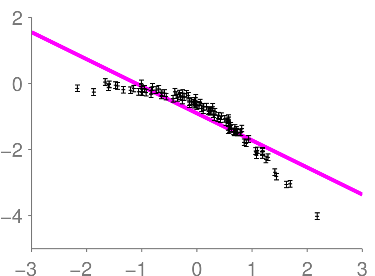
Here, we assumed a line model. But the given observations clearly follow a bent curve, so the line model is too simple. While it looks like there is just one line, we’ve drawn 12 lines from the posterior almost on top of each other, indicating that the posterior is sharply peaked.

A sharply peaked posterior represents a belief with low uncertainty. As a result, we can be very confident about properties of a model, even if running some checks (such as looking at residuals) would show that the model is obviously in strong disagreement with the data. Strong correlations between residuals is an indication for this being the case.

We can also have problems when we use a model that’s too complicated. As an extreme example for illustration, we could imagine fitting a function on \(x\!\in\![0,1]\) with a million RBFs spaced evenly over that range with bandwidths \(\sim10^{-6}\). We can closely represent any reasonable function with this representation. However, given (say) 20 observations, most of the basis functions will be many bandwidths away from all of the observations. Thus, the posterior distribution over most of the coefficients will be similar to the prior (check: can you see why?). Except at locations that are nearly on top of the observed data, our predictions will be nearly the same as under the prior. We will learn slowly with this model.

2 Simple cases of probabilistic model choice

Video: Bayesian model choice (21 minutes)
How to choose between Bayesian models using the marginal likelihood.

We have already used a simple form of probabilistic model comparison in Bayes classifiers. Given two fixed models \(p(\bx\g y\te1)\) and \(p(\bx\g y\te0)\), we could evaluate a feature vector under each and use Bayes’ rule to express our beliefs, \(P(y\g\bx)\), about which model the features came from.

With Gaussian class models, there are different ways that a model can win a comparison. If a model has a tight distribution, then it will usually be the most probable model when observations are close to its mean, even if those observations could also have come from a broad distribution centred nearby. On the other hand, broad distributions become the most probable model for extreme feature vectors or outliers. Finally, while the prior probabilities of the class models have some effect, the likelihoods of the models often dominate.

In the card game video, we talked about a nice example of comparing broad and narrow models is dice with different numbers of sides. If we told you that we chose a dice at random from a million-sided dice and a 10-sided dice and got a 5, you’d be pretty sure we’d rolled the 10-sided dice. That’s partly because of priors: you don’t think we could possibly own a million sided dice. But even if you thought that million-sided dice were just as common, you’d have the same view. For example, we could implement this game on a computer and show you the Python code:

from random import random
from math import floor
sides = [10, 1e6]
dice = (0.5 < random())
outcome = floor(random() * sides[dice]) + 1
outcome

Every time you see this code output a number between 1 and 10, you’ll assume that it came from dice=1. While it’s rare to get a small outcome like 5 with a million sided dice, it’s no rarer than any other outcome, such as 63,823. However, the small outcomes are more easily generated under the alternative narrow model, so it wins the comparison.

3 Application to regression models

Why do we usually favour a simple fit over the model with a million narrow basis functions described above? It could be because of priors: we might favour simple models. But actually the world is complicated, and our prior beliefs are that many functions have many degrees of freedom. What would happen if we gave half of our prior mass to the model with a million narrow basis functions? It would still usually lose a model comparison.

A regression model has to distribute its prior mass over all of the possible regression surfaces that it can represent, or over all of its parameters. If a model can represent many different regression surfaces, only some of these will match the data. The probability that a model \(\M\) assigns to some observations in a training set is: \[ p(\by\g X, \M) = \int p(\by, \bw\g X, \M) \intd\bw = \int p(\by \g X, \bw, \M)\,p(\bw\g\M) \intd\bw, \] where the parameters \(\bw\) are assumed unknown. Narrowly focussed models, where the mass of the prior distribution \(p(\bw\g\M)\) is concentrated on simple curves, will assign higher density to the outputs \(\by\) observed in many natural datasets than the million narrow basis function model. The narrow basis function model can model smooth functions, but can also fit highly oscillating data — it’s a broader model that can explain outliers, but that will usually lose to simpler models for well-behaved data.

The probability of the data under the model, given above, is the model’s marginal likelihood, and can be used to score different models, instead of a cross-validation score. For Gaussian models, and some other models (usually with conjugate priors, as discussed in the previous note), we can compute the integral. Later in the course we also discuss how to approximate marginal likelihoods, where we can’t solve the integral in closed form.

4 Application to hyperparameters

The main challenge with model-selection is often setting real-valued parameters like the noise level, the typical spread of the weights (their prior standard deviation), and the widths of some radial basis functions. These values are harder to cross-validate than simple discrete choices, and if we have too many of these parameters, we can’t cross-validate them all.

Incidentally, in the million narrow RBFs example, the main problem wasn’t that there were a million RBFs, it was that they were narrow. Linear regression will make reasonable predictions with many RBFs and only a few datapoints if the bandwidth parameter is broad and we regularize. So we usually don’t worry about picking a precise number of basis functions.¹

The full Bayesian approach to prediction was described in the previous note. We integrate over all parameters we don’t know. In a fully Bayesian approach, that integral would include noise levels, the standard deviation of the weights in the prior, and the widths of basis functions. Because the best setting of each of these values is unknown. However, computing integrals over all of these quantities can be difficult (we will return to methods for approximating such difficult integrals later in the course).

A simpler approach is to maximize some parameters, according to their marginal likelihood, the likelihood with most of the parameters integrated out. For example, in a linear regression model with prior \[ p(\bw\g \sigma_w) = \N(\bw; \mathbf{0}, \sigma_w^2\mathbb{I}), \] and likelihood \[ p(y\g \bx, \bw, \sigma_y) = \N(y; \bw^\top\bx, \sigma_y^2), \] we can fit the hyperparameters \(\sigma_w\) and \(\sigma_y\), parameters which specify the model, to maximize their marginal likelihood: \[ p(\by\g X, \sigma_w, \sigma_y) = \int p(\by, \bw\g X, \sigma_w, \sigma_y) \intd\bw = \int p(\by \g X, \bw, \sigma_y)\,p(\bw\g\sigma_w) \intd\bw. \] No held-out validation set is required.

Fitting a small number of parameters (\(\sigma_w\) and \(\sigma_y\)) to the marginal likelihood is less prone to overfitting than fitting everything (\(\sigma_w\), \(\sigma_y\), and \(\bw\)) to the likelihood \(p(\by \g X, \bw, \sigma_w, \sigma_y)\). However, overfitting is still possible.

5 Check your understanding

Can you work out how to optimize the marginal likelihood \(p(\by\g X,\sigma_w,\sigma_y)\) for a linear regression model? Look back at the initial note on Bayesian regression for results that could be useful. In that note we were assuming that the hyperparameters \(\sigma_w\) and \(\sigma_y\) were known and fixed. In the notation of that note, the marginal likelihood was simply \(p(\by\g X)\), because we didn’t bother to condition every expression on the hyperparameters. More guidance in the footnote².

6 Further Reading

Bishop Section 3.4 and Murphy Section 7.6.4 are on Bayesian model selection. For keen students, earlier sections of Murphy give mathematical detail for a Bayesian treatment of the noise variance.

For keen students: Chapter 28 of MacKay’s book has a lengthier discussion of Bayesian model comparison. Some time ago, Iain wrote a note discussing one of the figures in that chapter.

For very keen students: It can be difficult to put sensible priors on models with many parameters. In these situations it can sometimes be better to start out with a model class that we know is too simple, and only swap to a complex model when we have a lot of data. Bayesian model comparison can fail to tell us the best time to switch to a more complex model. The paper Catching up faster by switching sooner (Erven et al., 2012) has a nice language modelling example, and Iain’s thoughts are in the discussion of the paper.

For very keen students, Gelman et al.’s Bayesian Data Analysis book is a good starting point for reading about model checking and criticism. All models are wrong, but we want to improve parts of a model that are most strongly in disagreement with the data.