Gaussian Processes and Kernels

In this note we’ll look at the link between Gaussian processes and Bayesian linear regression, and how to choose the kernel function.

1 Bayesian linear regression as a GP

Video: Bayesian linear regression is a GP (19 minutes)
About the relation between Bayesian linear regression and Gaussian processes.

The Bayesian linear regression model of a function, covered earlier in the course, is a Gaussian process. If you draw a random weight vector \(\bw\sim \N(\mathbf{0},\sigma_w^2 \I)\) and bias \(b\sim \N(0,\sigma_b^2)\) from Gaussians, the joint distribution of any set of function values, each given by \[ f(\bx^{(i)}) = \bw^\top\bx^{(i)} + b, \] is Gaussian. If the distributions over the weights are prior beliefs, then we are specifying a Gaussian process prior on a function.

A Gaussian Process created by a Bayesian linear regression model is degenerate (boring), because the function has to be linear in \(\bx\). Once we know the function at \((D+1)\) input locations (assuming locations in general position to avoid exotic cases), we can solve for the weights, and we know the function everywhere. If we use \(K\) basis functions, the function is constrained to be a linear combination of those basis functions. Knowing the function at only \(K\) positions is usually enough to find the basis functions’ coefficients and know the function everywhere.

By choosing an appropriate kernel function, we can define Gaussian processes that are more interesting. The covariance matrices we produce can be full rank, which would mean that no matter how many function values we see, there would still be more to learn about the function.

2 Bayesian linear regression’s kernel

As Bayesian linear regression defines a Gaussian process, there is a corresponding kernel function that specifies all of the covariances in the model: \[ \begin{align} \tilde{f}_i &\,=\, f(\bx\ith) \,=\, \bw^\top \bx\ith + b, \qquad \bw\sim \N(\mathbf{0}, \sigma_w^2\eye), \,~ b\sim \N(0, \sigma_b^2)\\ \mathrm{cov}(\tilde{f}_i, \tilde{f}_j) &\,=\, \mathbb{E}[\tilde{f}_i \tilde{f}_j] - \overbrace{\mathbb{E}[\tilde{f}_i]\mathbb{E}[\tilde{f}_j]}^0\\ &\,=\, \mathbb{E}\big[ (\bw^\top \bx\ith + b)^\top (\bw^\top \bx\jth+ b) \big]\\ &\,=\, \sigma_w^2 \bx^{(i)\top} \bx\jth + \sigma_b^2 \,=\, {k(\bx\ith,\bx\jth)}. \end{align} \] The kernel is specified by parameters \(\sigma_w^2\) and \(\sigma_b^2\), which are hyperparameters in a Bayesian hierarchical model — parameters that specify the prior on parameters.

It’s usually more efficient to implement Bayesian linear regression directly, than interpreting it as a Gaussian process. Although if there are more input features or basis functions than data-points, using the Gaussian process view is cheaper.

3 Feature spaces and the kernel trick

We can replace the original features \(\bx\) with a vector of basis function evaluations \(\bphi(\bx)\) in the linear regression model. We obtain the kernel: \[ k(\bx\ith,\bx\jth) = \sigma_w^2 \bphi(\bx^{(i)})^\top\bphi(\bx\jth) + \sigma_b^2. \] To get arbitrarily complicated functions, we would need an infinite \(\bphi\) vector of features. Fortunately, all we need to know are inner products \(\bphi(\bx^{(i)})^\top\bphi(\bx^{(j)})\) — the feature vector never occurs by itself in the maths. If we can get the inner products directly, without creating the infinite feature vectors, we can infer an infinitely complicated model, with a finite amount of computation.

Replacing an inner product of features with a simple kernel function, corresponding to a large or infinite set of basis functions, is known as the kernel trick. Some kernels are derived explicitly as inner products of an infinite collection of basis functions. Moreover, it can be shown that Mercer kernels, or positive definite kernels, all correspond to taking inner products in some feature space, which might be infinite.

Several other machine learning algorithms can be expressed in terms of only inner products, and so can be kernelized. Later in the course, we will encounter a method for dimensionality reduction known as Principal Components Analysis (PCA) that can be written using only inner products. Most famously, a linear classifier known as the Support Vector Machine (SVM) is usually used in its kernelized version. Gaussian processes are kernelized Bayesian linear regression.

4 Choosing a family of kernel functions

Video: Learning the kernel (19 minutes)
Some intuition about Gaussian processes and how to learn the kernel.

We can’t just make up any function for \(k(\bx\ith,\bx\jth)\). We have to know that it will always give positive semi-definite matrices (and usually we want positive definite matrices), so that the prior on functions is actually a valid Gaussian distribution.

The textbooks have various options, and we won’t go through them all. We’ll briefly highlight some of the things that are worth knowing.

Going beyond feature vectors: There are kernel functions that can compare two strings or graphs, and return a covariance. Kernel methods give a flexible means to model functions of structured objects.

Kernels can be combined in various ways. For example, given two positive definite kernel functions, a positive combination: \[ k(\bx\ith, \bx\jth) = \alpha k_1(\bx\ith, \bx\jth) + \beta k_2(\bx\ith, \bx\jth), \quad \alpha>0,~\beta>0, \] is also positive definite. (Can you prove it?)

Kernels can give functions with qualitatively different properties: The examples in these notes come from Gaussian kernels. The functions from this prior are ridiculously smooth for many purposes, and other choices may be better. (In high-dimensions you can’t really see any detail of a function, and the smoothness of the Gaussian kernel probably matters less.)

Kernels usually have parameters. Most kernels have free parameters that change the distribution over functions. The combination of kernels above introduced two extra parameters \(\alpha\) and \(\beta\). As explained above, the link to Bayesian linear regression means that these parameters are often called hyperparameters. Tuning hyperparameters is the main way that we control the prior of a Gaussian process. The choice of prior strongly affects the model’s generalization performance for a given amount of data.

5 Hyperparameters for the Gaussian kernel

The Gaussian kernel can be derived from a Bayesian linear regression model with an infinite number of radial-basis functions. You might see several other names for the kernel, including RBF, squared-exponential, and exponentiated-quadratic.

The version below has hyperparameters \(\sigma_f\), \(\ell_d\) to control its properties, \[ k(\bx\ith, \bx\jth) \;=\; \sigma_f^2\, \exp\!\bigg(\!-{\textstyle\frac{1}{2}} \sum_{d=1}^D (x_d\ith - x_d\jth)^2 / \ell_d^2 \bigg). \] Other kernels have similar parameters, but we will demonstrate their effect just on the Gaussian kernel.

The marginal variance of one function value \(\tilde{f}_i\) is: \[ \text{var}[\tilde{f}_i] = k(\bx\ith,\bx\ith) = \sigma_f^2. \] The figure below illustrates functions drawn from priors with different marginal variances, also called “function variance” or “signal variance”, \(\sigma_f^2\):

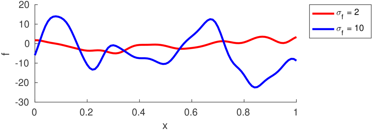
If we saw a long enough stretch of function, then \(\approx\frac{2}{3}\) of the points would be within \(\pm\sigma_f\) of the mean (which is zero in all the figures here). Although we often won’t see long stretches of a function with many turning points.

The number of turning points in the function is random, but controlled by the lengthscale \(\ell\). (Some papers refer instead to a “bandwidth” \(h\), as was traditionally used with RBF models, but is less used with GPs.) As in the equation above, each feature dimension might have its own lengthscale \(\ell_d\), or there might be a single shared lengthscale \(\ell\). The plot below illustrates samples with two different lengthscales:

The lengthscale indicates the typical distance between turning points in the function. Often a good value is comparable to the range of a feature in the training data, because functions in many regression problems don’t have many turning points.

6 Learning the hyperparameters

If we observe \(\by\) a vector of function values with Gaussian noise added, the probability of the data is just a Gaussian. The log of that probability is the log of the standard multivariate Gaussian pdf: \[ \log p(\by\g X,\theta) = -{\textstyle\frac{1}{2}} \by^\top M^{-1}\by - {\textstyle\frac{1}{2}} \log\left|M\right| - {\textstyle\frac{N}{2}}\log 2\pi, \] where \(M = K + \sigma_y^2\I\), is the kernel matrix evaluated at the training inputs plus the variance of the observation noise. The model hyperparameters \(\theta\) are the kernel parameters \(\{\ell_d, \sigma_f, \dots\}\), which control \(K\), and the noise variance \(\sigma_y^2\).

One way to set the hyperparameters is by maximum likelihood: find values that make the observations seem probable. Because the GP can be viewed as having an infinite number of weight parameters that have been integrated or marginalized out, \(p(\by\g X,\theta)\) is often called the marginal likelihood.

Optimizing the marginal likelihood of a stochastic process sounds fancy. But all we are doing is fitting a Gaussian distribution (albeit a big one) to some data, and the marginal likelihood is just the usual pdf for a Gaussian. A minimal implementation isn’t much code. We can use a grid search, as when optimizing hyperparameters on a validation set. However, an advantage of the marginal likelihood is that it’s easy to differentiate. When we have many parameters we can use gradient-based optimizers (a practical detail is discussed in the next note).

It is quite possible to overfit when fitting the hyperparameters. Regularizing the log noise variance \(\log\sigma_y^2\), to prevent it from getting too small, is often a good idea.

A fully Bayesian approach is another way to avoid overfitting. It computes the posterior over a function value by integrating over all possible hyperparameters: \[ p(f_*\g \by,X) = \int p(f_*\g \by,X,\theta)\, p(\theta\g \by,X)\; \mathrm{d}\theta \] However, this integral can’t be computed exactly. The first term in the integrand is tractable. The second term is the posterior over hyperparameters, which comes from Bayes’ rule, but must be approximated before we can compute the integral.

7 Computation cost and limitations

Gaussian processes show that we can build remarkably flexible models and track uncertainty, with just the humble Gaussian distribution. In machine learning they are mainly used for modelling expensive functions. But they are also used in a large variety of applications in other fields (sometimes under a different name).

The main downside to straightforward Gaussian process models is that they scale poorly with large datasets.

• The \(O(N^3)\) computation cost usually takes the blame, required to factor the \(M\) matrix above so that we can evaluate the marginal likelihood and make predictions.
• That cost isn’t the only story. Computing the kernel matrix costs \(O(DN^2)\) and uses \(O(N^2)\) memory. Sometimes the covariance computations can be significant, and running out of memory places a hard limit on practical problem sizes.
• There is a large literature on special cases and approximations of GPs that can be evaluated more cheaply.

Not all functions can be represented by a Gaussian process. The probability of a function being monotonic is zero under any Gaussian process with a strictly positive definite kernel.

Gaussian processes are a useful building block in other models. But as soon as our observation process isn’t Gaussian, we have to do rather more work to perform inference, and we need to make approximations.

8 Check your understanding

What distributions are \(\sigma_f^2\) and \(\sigma_y^2\) the variances of?

Below are additional questions about the lengthscale parameter(s) \(\ell_d\) in the Gaussian kernel. You should think about what the prior model says, and so reason about what will be imposed on the posterior.

• What will happen as the lengthscale \(\ell\) is driven to infinity?

• If a kernel has a different lengthscale \(\ell_d\) for each feature-vector dimension, what happens if we drive one of these lengthscales to infinity?

9 Further Reading

The readings from the previous note still stand.

Carl Rasmussen has a nice example of how GPs can combine multiple kernel functions to model interesting functions:
http://learning.eng.cam.ac.uk/carl/mauna/

Some Gaussian process software packages:

• https://gpytorch.ai/
  Uses GPU acceleration and PyTorch but new and in development.
• https://github.com/GPflow/GPflow
  Uses automatic differentiation and TensorFlow, also new and in development.
• https://sheffieldml.github.io/GPy/
  More mature Python codebase.
• http://www.gaussianprocess.org/gpml/code/matlab/doc/
  Nicely structured Matlab code base. (Used in Carl’s demo above.)
• https://research.cs.aalto.fi/pml/software/gpstuff/
  Matlab. Less easy-to-follow code, but implements some interesting things.
• https://sheffieldml.github.io/GPyOpt/
  Bayesian optimization based on GPy.¹

Those who want to read more about the theory of the kernel trick, and why a positive-definite kernel always corresponds to inner-products in some feature space, could read section 2.2 of: “Learning with kernels: Support Vector Machines, Regularization, Optimization, and Beyond”, Bernhard Schölkopf and Alexander J. Smola. Section 16.3 of this book is on Gaussian processes specifically.

10 Practical tips

As with any machine learning method, the machines can’t do everything for us yet. Visualize your data. Look for weird artifacts that might not be well captured by the model. Consider how to encode inputs (one-hot encoding, log-transforms, …) and outputs (log-transform? …).

To set initial hyperparameters, use domain knowledge wherever possible. Otherwise…

• Standardize input data and set (initial) lengthscales \(\ell_d\) to \(\sim 1\).
• Standardize targets and set the function variance \(\sigma_f^2\) to \(\sim 1\).
• Sometimes useful: set the initial noise level high, even if you think your data have low noise. The optimization surface for your other hyperparameters will be easier to move in.

If optimizing hyperparameters, (as always) random restarts or other tricks to avoid local optima may be necessary.

Don’t believe any suggestions that maximizing marginal likelihood can’t overfit. It can, so watch out for it, and consider more Bayesian alternatives.