Autoencoders and Principal Components Analysis (PCA)
One of the purposes of machine learning is to automatically learn how to use data, without writing code by hand. When we started the course with linear regression, we saw that we could represent complicated functions if we hand-engineered features (or basis functions). Those functions can then be turned into “neural networks”, where — given enough labelled data — we can learn the features that are useful for classification automatically.
For some data science tasks the amount of labelled data is small. In these situations it is useful to have pre-existing basis functions that were fitted as part of solving some other task. We can then fit a linear regression model on top of these basis functions. Or perhaps use the basis functions to initialize a neural network, and only train for a short time.
The basis functions could come from fitting another supervised task. For example, neural networks trained on the large ImageNet dataset are often used to initialize the training of image recognition models for tasks with only a few labels.
We may also wish to use completely unlabelled data, such as relevant but unannotated images or text. Recently (2018–), there has been an explosion of interest in Natural Language Processing in using pre-trained deep neural networks based on unlabelled data. See the Further Reading for papers.
1 Autoencoders
Video: Autoencoders (32 minutes)
Autoencoders are neural networks that “predict” their own input. We discuss autoencoders that do dimensionality reduction, and ones that learn high-dimensional sparse features.
Autoencoders solve an “unsupervised” task: find a representation of feature vectors, without any labels. This representation might be useful for other tasks. An autoencoder is a neural network representing a vector-valued function, which when fitted well, approximately returns its input: \[ \bff(\bx) \approx \bx. \] If we were allowed to set up the network arbitrarily, this function is easy to represent. For example, we could use a single “weight matrix”: \[ \bff(\bx) = W\bx, \quad \text{with}~W=\I,~\text{the identity}. \] Constraints are required to find an interesting representation that might be useful.
Dimensionality reduction: One possible constraint is to form a “bottleneck”. We use a neural network with a narrow hidden layer with \(K\ll D\) units: \[\begin{align} \bh &= g^{(1)}(W^{(1)}\bx + \bb^{(1)})\\ \bff &= g^{(2)}(W^{(2)}\bh + \bb^{(2)}), \end{align}\] where \(W^{(1)}\) is a \(K\ttimes D\) weight matrix, and the \(g\)’s are element-wise functions. If the function output manages to closely match its inputs, then we have a good lossy compressor. The network can compress \(D\) numbers down into \(K\) numbers, and then decodes them again, approximately reconstructing the original input.
One application of dimensionality reduction is visualization. When \(K\te2\) we can plot our transformed data as a 2-dimensional scatter-plot.
When an autoencoder works well, the transformed values \(\bh\) contain most of the information from the original input. We should therefore be able to use these transformed vectors as input to a classifier instead of our original data. It might then be possible to fit a classifier using less labelled data, because we are fitting a function with lower-dimensional inputs.
Fitting the weights of an autoencoder extracts information about how our inputs are distributed from our training dataset, which might help us fit a classifier or other methods. However, at test time, transforming an individual input with an autoencoder can’t add information about that example, an observation known as the “data processing inequality”.
Denoising and sparse autoencoders: Fitting an autoencoder with a high-dimensional hidden layer gives features that are easier to separate with a linear classifier.1 A regularization strategy that enables setting \(K\!\ge\!D\) is the denoising autoencoder: randomly set some of the features in the input to zero, but try to reconstruct the original uncorrupted vector. Then if \(K\te D\) the best strategy is no longer for \(W^{(1)}\) to be the identity matrix. The hidden units should represent common conjunctions of multiple input features, so that missing features can be reconstructed. Alternatively, sparse autoencoders only allow a small fraction of the \(K\) hidden units to take on non-zero values. That limitation forces the network to represent the input vector as a linear combination of a small number of different “sources”. A large number, \(K\), of different sources are possible, but only a few can be used for each example.
2 Interlude on covariance matrices
Real symmetric matrices, like covariance matrices, can be decomposed as: \[ \Sigma = Q\Lambda Q^\top, \] where \(\Lambda\) is a diagonal matrix containing the eigenvalues of \(\Sigma\), and the columns of \(Q\) contain the eigenvectors of \(\Sigma\).
Questions:
Describe how to sample from \(\N(\mathbf{0},\Sigma)\) given \(Q\) and \(\Lambda\).
Hint: If you can write the covariance in the form \(\Sigma = AA^\top\), you should have the answer.
You may not just recompute \(\Sigma = Q\Lambda Q^\top\) and then use some other decomposition, like the Cholesky decomposition; you need to actually use the eigendecomposition!
\(Q\) is an orthogonal matrix, corresponding to a rigid rotation (and possibly a reflection). Describe geometrically (perhaps in 2D) how the sampling process in part a) transforms a cloud of points drawn from a standard normal.
Hint: consider what happens to a point sitting one unit along one of the axes, e.g. at (1, 0) in 2D.
3 Principal Components Analysis (PCA)
Video: Principal Components Analysis, PCA (29 minutes)
We describe PCA as a linear autoencoder, show three example applications, and mention the importance of pre-processing. (Not mentioned: you should also remember other pre-processing tricks like log-transforming +ve quantities, and one-hot encoding.)
Video: PCA more maths detail (9 minutes)
Discussion of how the eigenvectors of the covariance are used in PCA, and how finding directions with the highest variance minimizes square reconstruction error. May help follow the proofs in the textbooks.
A linear autoencoder sets the activation functions above to \(g^{(1)}(a) = g^{(2)}(a) = a\). It turns out that2 the best square error for a linear auto-encoder can still be obtained when re-writing the transformations in the restricted form: \[\begin{align} \bh &= W^{(1)}\bx + \bb^{(1)} = V^\top(\bx -\bar{\bx})\\ \bff &= W^{(2)}\bh + \bb^{(2)} = V\bh + \bar{\bx}. \end{align}\] The first step centres the input by subtracting the mean \(\bar{\bx} = \frac{1}{N} \sum_n \bx\nth\), and then transforms to a \(K\)-dimensional ‘hidden’ representation using a \(D\ttimes K\) matrix \(V\). The second step transforms back up to the high \(D\)-dimensional space, and re-centres the points around the mean. The parameters in the two transformations are shared, which turns out not to be a limitation.
The method of Principal Components Analysis (PCA) identifies a matrix \(V\), which if used in the above autoencoder achieves the best possible square error. There are three advantages over fitting the autoencoder with gradient methods: 1) The solutions for different hidden layer sizes \(K\) are nested: for a given input vector, the extracted feature \(h_1\) is the same in the solutions for all \(K\), \(h_2\) is the same for all \(K\!\ge\!2\), and so on. 2) This constraint makes the solution unique, so we fit the same parameters every time. 3) The parameters can be found using standard linear algebra operations.
We compute the covariance matrix of the points \(\Sigma = \frac{1}{N}\sum_n (\bx\nth-\bar{\bx})(\bx\nth-\bar{\bx})^\top\). Recalling the material on multivariate Gaussians, the covariance can be used to describe an ellipsoidal ball that summarizes how the data is spread in space.3 Some axes of the ellipsoid are often very short, and the data is “squashed” into a ball that only significantly extends in some directions. As we saw in the interlude on covariances above, the eigenvectors of the covariance matrix point along the axes of the ellipsoid, and the longest axes are the eigenvectors with the largest eigenvalues.
PCA measures the displacement of a data-point from the mean \(\bar{\bx}\) along the \(K\) most elongated axes of the ellipsoid. To do that, it sets the columns of the transformation matrix \(V\) to the \(K\) eigenvectors of the covariance matrix associated with the largest \(K\) eigenvalues.
Example Python code:
# Find top K principal directions:
E, V = np.linalg.eig(np.cov(X.T))
idx = np.argsort(E)[::-1]
V = V[:, idx[:K]]  # (D,K)
x_bar = np.mean(X, 0)

# Transform down to K-dims:
X_kdim = np.dot(X - x_bar, V)  # (N,K)

# Transform back to D-dims:
X_proj = np.dot(X_kdim, V.T) + x_bar  # (N,D)
An illustration for \(D\te2\) and \(K\te1\):
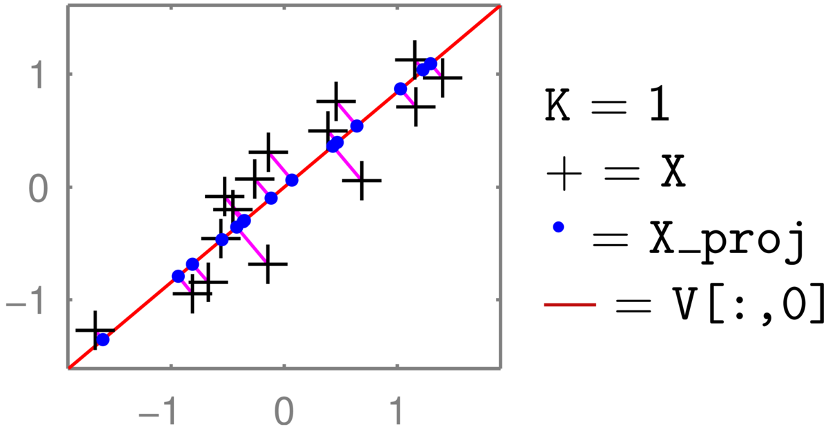
The two-dimensional coordinate of each \(+\) is reduced to one number, giving the position along the red line that it has been projected onto (the principal component). Transforming back up to two dimensions gives the coordinates of the \(\bullet\)’s in the full 2-dimensional space. These projected points (for zero-mean data \(XVV^\top\)) are constrained to lie along a one-dimensional line. (See also the related discussion in Q5 of the background material self-test.) The position along the second principal axis has been lost.
The eigenvectors of a covariance matrix are orthogonal, so if all the dimensions are kept, that is \(K\te D\), then \(VV^\top = \I\), and no information is lost.
We can replace a feature vector \(\bx\) with a linear transformation \(A\bx\) in any model. The transformation \(A\) could even be generated at random (no fitting, so no risk of overfitting!). Alternatively the transformation could be seen as \(K\ttimes D\) extra parameters, and fitted as part of the model (like in a neural network). PCA is a way to fit a sensible transformation, but without fitting (and possibly overfitting) to a specific task.
4 PCA Examples
PCA is widely used, across many different types of data. It can give a quick first visualization of a dataset, or reduce the number of dimensions of a data matrix if overfitting or computational cost are concerns.
An example where we expect data to be largely controlled by a few numbers is body shape. The location of a point on a triangular mesh representing a human body is strongly constrained by the surrounding mesh-points, and could be accurately predicted with linear regression. PCA describes the principal ways in which variables can jointly change when moving away from the mean object.4 The principal components are often interpretable, and can be animated. Starting at a mean body mesh, one can move along each of the principal components, showing taller/shorter people, and then thinner/fatter people. The later principal components will correspond to more subtle, less interpretable combinations of features that covary.
A striking PCA visualization was obtained by reducing the dimensionality of \(\approx 200,000\) features of people’s DNA to two dimensions (Novembre et al., 2008).5 The coordinates along the two principal axes closely correspond to a map of Europe showing where the people came from(!). The people were carefully chosen.
As is often the case with useful algorithms, we can choose how to put our data into them, and solve different tasks with the same code. Given an \(N\ttimes D\) matrix, we can run PCA to visualize the \(N\) rows. Or we can transpose the matrix and instead visualize the \(D\) columns. As an example, we took a binary \(S\ttimes C\) matrix \(M\) relating students and courses. \(M_{sc} \te 1\), if student \(s\) was taking course \(c\). In terms of these features, each course is a length-\(S\) vector, or each student is a length-\(C\) vector. We can reduce either of these sets of vectors to 2-dimensions and visualize them.
The 2D scatter plot of courses was somewhat interpretable:
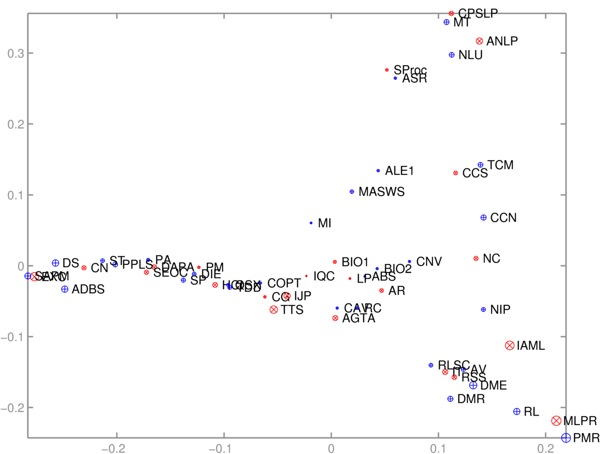
One axis (roughly) goes from computer-based applications of Informatics, through theory to broader applications. The other goes from cognitive/language applications down to machine learning. The algorithm had no labels, just which courses are taken together.
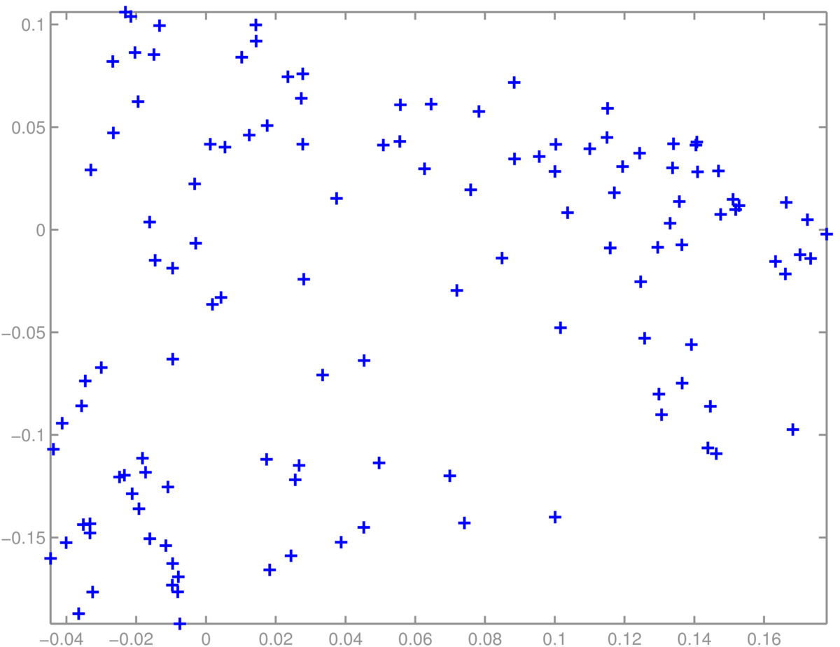
A scatter plot of students was less interpretable. We didn’t find obvious groups corresponding to the topics (suggested groups of courses) in the Informatics MSc handbook:
Finally, PCA doesn’t always work well. One of the papers that helped convince people that it was feasible to fit deep neural networks showed impressive results with non-linear deep autoencoders in cases where PCA worked poorly: Reducing the dimensionality of data with neural networks, Hinton and Salakhutdinov (2006). Science, Vol. 313. no. 5786, pp504–507, 28 July 2006. Available from https://www.cs.utoronto.ca/~hinton/papers.html
5 Pre-processing matters
The units that data are measured in affects the principal components. Given age, weights, and heights of people, it matters if their height is measured in centimeters or meters. The numbers are 100 times bigger if we use centimeters, making the square error for an equivalent mistake in reconstructing height 10,000 times bigger. Therefore, if we use centimeters the principal component will be more aligned with height to reduce overall square error than if we use meters. To give each feature similar importance, it’s common to standardize all features so they have unit standard deviation: but the best scaling could depend on the application.
Given DNA data, \(x_d \in \{\mathtt{A},\mathtt{C},\mathtt{G},\mathtt{T}\}\), we have to decide how to encode categorical data. We could use one-hot encoding. In the example above, Novembre et al. used a lossy binary encoding indicating if the subject had the most common letter or not.
As usual, given positive data, we may wish to take logarithms. There are lots of free choices in data analysis.
6 PCA and SVD
Video: Singular Value Decomposition, SVD for PCA (8 minutes)
SVD is a standard matrix decomposition that can be used to approximate data matrices and implement PCA.
The truncated SVD view of PCA reflects the symmetry noted in the MSc course data example above: we can find a low-dimensional vector representing either the rows or columns of a matrix. SVD finds both at once.
The truncated Singular Value Decomposition (SVD) is a standard technique, available in most linear algebra packages. It approximates an \(N\ttimes D\) matrix as a product of three matrices, \[ X \approx U S V^\top, \] where \(U\) has size \(N\ttimes K\), \(S\) is a diagonal \(K\ttimes K\) matrix, and \(V^\top\) has size \(K\ttimes D\). The columns of the \(V\) matrix (or the rows of \(V^\top\)) contain eigenvectors of \(X^\top X\). The columns of \(U\) contain eigenvectors of \(XX^\top\). The rows of \(U\) give a \(K\)-dimensional embedding of the rows of \(X\). The columns of \(V^\top\) (or the rows of \(V\)) give a \(K\)-dimensional embedding of the columns of \(X\).
When \(K \te \min(N, D)\), SVD exactly reconstructs the matrix. For smaller \(K\), truncated SVD is known to be the best low-rank approximation of a matrix, as measured by square error.
When applied to centred data (the mean feature vector has been subtracted from every row of \(X\), so that \(\sum_n X_{nd} \te 0\) for each feature \(d\)), SVD gives the same solution as PCA. The \(V\) matrix contains the eigenvectors of the covariance (\(\Sigma = \frac{1}{N}X^\top X\), where the \(1/N\) scaling makes no difference to the directions). The \(U\) matrix contains the eigenvectors of the covariance if we were to transpose our data matrix before applying PCA.
Python demo:
# PCA via SVD, for NxD matrix X
x_bar = np.mean(X, 0)
[U, vecS, VT] = np.linalg.svd(X - x_bar, 0) # Apply SVD to centred data
U = U[:, :K] # NxK "datapoints" transformed into K-dims
vecS = vecS[:K] # The diagonal elements of diagonal matrix S, in a vector
V = VT[:K, :].T # DxK "features" transformed into K-dims
X_kdim = U * vecS # = np.dot(U, np.diag(vecS))
X_proj = np.dot(X_kdim, V.T) + x_bar # SVD approx USV' + mean
7 Probabilistic versions of PCA
Video: Gaussian models for PCA (10 minutes)
Building up the Gaussian model for Probabilistic PCA and Factor Analysis.
The simplest probabilistic model of \(D\)-dimensional feature vectors \(\bx\) that lie on a low-dimensional manifold, is to assume they’re Gaussian. The model assumes that a \(K\)-dimensional Gaussian variable was generated, \(\bnu \sim \N(\mathbf{0},\I_K)\), and then transformed up into \(D\)-dimensions, \(\bx = W\bnu + \bmu\), where \(W\) is a \(D\ttimes K\) matrix. Under this model, \(\bx \sim \N(\bmu,\, WW^\top)\). The covariance is low rank, rank \(K\), because it only has \(K\) independent rows or columns. By the construction, all vectors \(\bx\) generated from this model will lie exactly on a linear subspace of dimension \(K\).
A Gaussian with low-rank covariance isn’t able to explain real-world data, which won’t lie exactly on a linear subspace. Specifically the likelihood of such a model will be zero if any data-points lie outside the \(K\)-dimensional subspace. We can explain such deviations by assuming that spherical noise was added to the points from the model of the previous paragraph: \(\bx \sim \N(\bmu,\, WW^\top \!+ \sigma^2\I)\). This is the probabilistic PCA (PPCA) model. In the limit as \(\sigma^2\rightarrow 0\) the low-dimensional explanations of the data will be the same as PCA. But a more sensible model will result by setting non-zero \(\sigma^2\). PPCA is a special case of probabilistic Factor Analysis, which sets the noise to be an arbitrary diagonal covariance matrix.
8 Further reading
Different tutorials will focus on different use-cases of PCA. Some practitioners are mostly interested in reducing the dimensionality of their data. Others are interested in inspecting and interpreting the components.
You may also find that different tutorials put different emphasis on the two different principles from which PCA can be derived: 1) Auto-encoding / error minimization: PCA provides the nested set of \(K\)-dimensional linear subspaces that minimize square error when reconstructing the data with a linear transformation. 2) Variance maximization: each principal component is the direction in which the data is most spread out (as measured by the variance), with the constraint that each component is orthogonal to all of the previous components. It’s neat that these two different principles give the same principal components!
Bishop covers PCA in Chapter 12, with mathematical detail to back up the results.
Murphy’s treatment of PCA: Section 12.2.1 p387–389, and Section 12.2.3 pp392–395.
Barber’s treatment starts in Section 15.2.
There are many online tutorials about PCA, with different levels of detail. The one by Alex Williams looks good.
Goodfellow et al.’s Deep Learning Textbook has much more on autoencoders in Chapter 14.
If you wanted to train an auto-encoder to have a nested set of hidden units like PCA, where keeping the top \(K\) units gives good reconstructions, you could use a method called “Nested Dropout” (Rippel et al, 2014).
There are also non-parametric dimensionality reduction methods for visualization, such as t-SNE. These place each data-point at an arbitrary location on a scatter plot, by minimizing a cost function. The cost function says it is good if some properties of the scatter plot match the original high-dimensional data. For example, it is good to approximately preserve the relative distances between points, especially between nearby-points. There are examples where t-SNE gives far better visualizations than PCA does. I’ve also recently (2018) enjoyed using UMAP. However, in other applications (like the MSc data above) the best method of several I tried was simple linear PCA.
We can modify a denoising autoencoder to only compute the loss on the predictions of features that were masked out. It’s possible to turn such a network into a probabilistic model \(P(\bx)\) of the inputs6. Such masked autoencoder objectives have also been used in BERT (Devlin et al., 2018)7, to pre-train representations of text for use in many other Natural Language Processing (NLP) tasks. BERT and its successors are causing big changes in NLP8, including (October 2019) how Google search works9.
9 Bonus note on matrix functions
Non-examinable!
A previous MLPR student asked: if \(X\) is a square symmetric matrix, doesn’t the SVD of \(X\) give us the eigenvectors of \(X\)? Yes it does. That’s potentially confusing because above we said that the SVD gives the eigenvectors of \(XX^\top\) and \(X^\top X\). For a square symmetric matrix, the SVD therefore gives the eigenvectors of \(X^2\). These are in fact the same as the eigenvectors of \(X\), so there’s no contradiction.
\(X^2\) is the square function applied to the matrix \(X\). A way to apply a function to a square matrix is to decompose the matrix using its eigendecomposition \(X = U \Lambda U^{-1}\), apply the function to the diagonal elements of \(\Lambda\) (in this case square the values), and then put the matrix back together again. The eigenvectors don’t change! For a square symmetric matrix, the SVD and the eigendecomposition are the same thing.
It may interest you to know that other functions are applied to matrices in this way. For example the matrix exponential of a square matrix (scipy.linalg.expm in Python), equal to \(X+\frac{1}{2}X^2 + \frac{1}{3!}X^3 + \frac{1}{4!}X^4+\ldots\), can (in principle) be computed by taking the eigendecomposition, exponentiating the eigenvalues, and putting the matrix back together again. (Although the best way to compute the matrix exponential numerically is a complicated question.)
This animation: https://www.youtube.com/watch?v=3liCbRZPrZA demonstrates a non-linear transformation of two-dimensional points into three dimensions. In this example, a circle of points in a two dimensional space can be separated with a plane in a three-dimensional space.↩︎
We don’t prove any of the properties of PCA in this note. We sketch some of the theory in slightly more detail in the video, but see the (optional) further reading for detailed proofs if you want them.↩︎
The data might not be Gaussian distributed, so this summary could be misleading, just as the standard deviation can be a misleading indicator of width for a 1D distribution.↩︎
While they’re doing something a little more complicated, you can get an idea of what the principal components of body shape look like from the figures in the paper: Lie bodies: a manifold representation of 3D human shape, Freifeld and Black, ECCV 2012.↩︎
Genes mirror geography within Europe. https://www.nature.com/articles/nature07331↩︎
https://blog.google/products/search/search-language-understanding-bert↩︎