Write a numbered list of the three most interesting things that you observed while peforming your experiments in the w7a check your understanding section.
Each of your points should only be one or two sentences. While we hope that you found out more than three things, please do not list more than three.
Please compare your answers in your tutorial. In particular, discuss anything that you found surprising or confusing.
Learning a transformation:
The \(K\)-nearest-neighbour (KNN) classifier predicts the label of a feature vector by finding the \(K\) nearest feature vectors in the training set. The label predicted is the label shared by the majority of the training neighbours. For binary classification we normally choose \(K\) to be an odd number so ties aren’t possible.
KNN is an example of a non-parametric method: no fixed-size vector of parameters (like \(\bw\) in logistic regression) summarizes the training data. Instead, the complexity of the function represented by the classifier grows with the number of training examples \(N\). Often, the whole training set needs to be stored so that it can be consulted at test time. (Gaussian processes are also a non-parametric method.)
- How would the predictions from regularized linear logistic regression, with \(P(y\te1\g\bx,\bw,b) = \sigma(\bw^\top\bx+b)\), and 1-nearest neighbours compare on the dataset below?
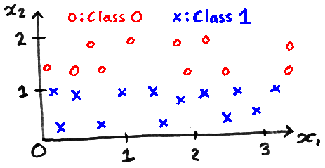
Non-parametric methods can have parameters. We could modify the KNN classifier by taking a linear transformation of the data \(\bz = A\bx\), and finding the \(K\) nearest neighbours using the new \(\bz\) features. We’d like to learn the matrix \(A\), but for \(K\te1\), the training error is 0 for almost all \(A\) (the nearest neighbour of a training point is itself, which has the correct label by definition).
A loss function that could evaluate possible transformations \(A\) is the leave-one-out (LOO) classification error, defined as the fraction of errors made on the training set when the \(K\) nearest neighbours for a training item don’t include the point being classified itself.
The identity transformation, which does nothing, is: \[A = \begin{bmatrix} 1 & 0\\ 0 & 1\\ \end{bmatrix}. \] Write down a matrix \(A\) where the 1-nearest neighbour classifier has lower LOO error than using the identity matrix for the data above. Explain why your matrix works in about three sentences.
Explain whether we can fit the LOO error for a KNN classifier by gradient descent on the matrix \(A\).
Assume that I have implemented some other classification method where I can evaluate a cost function \(c\) and its derivatives with respect to feature input locations: \(\bar{Z}\), where \(\bar{Z}_{nk} = \pdd{c}{Z_{nk}}\) and \(Z\) is an \(N\ttimes H\) matrix of inputs.
I will use that code by creating the feature input locations from a linear transformation of some original features \(Z = XA^\top\). How could I fit the matrix \(A\)? If \(A\) is an \(H\ttimes D\) matrix, with \(H\!<\!D\), how will the computational cost of this method scale with \(D\)?
You may quote results given in lecture note w7d.
Linear autoencoder
We centre our data so it has zero mean, and fit a linear autoencoder with no bias parameters. The autoencoder is a \(D\)-dimensional vector-valued function \(\bff\), computed from \(D\)-dimensional inputs \(\bx\), using an intermediate \(K\)-dimensional “hidden” vector \(\bh\): \[\begin{align} \notag \bh &= W^{(1)}\bx\\ \notag \bff &= W^{(2)}\bh. \end{align}\] Assume we want to find a setting of the parameters that minimizes the square error \(\|\bff-\bx\|^2 = (\bff - \bx)^\top(\bff-\bx)\), averaged (or summed) over training examples.
What are the sizes of the weight matrices \(W^{(1)}\) and \(W^{(2)}\)? Why is it usually not possible to get zero error for \(K\!<\!D\)?
It’s common to transform a batch (or “mini-batch”) of data at one time. Given an \(N\ttimes D\) matrix of inputs \(X\), we set: \[\begin{align} \notag H &= XW^{(1)\top}\\ \notag F &= HW^{(2)\top} \end{align}\] The total square error \(E = \sum_{nd} (F_{nd} - X_{nd})^2\), has derivatives with respect to the neural network output \[\notag \pdd{E}{F_{nd}} = 2(F_{nd} - X_{nd}), \quad \text{which we write as}~ \bar{F} = 2(F - X). \] Using the backpropagation rule for matrix multiplication, \[\notag C = AB^\top \quad\Rightarrow\quad \bar{A} = \bar{C}B ~~\text{and}~~ \bar{B} = \bar{C}^\top A, \] write down how to compute derivatives of the cost with respect to \(W^{(1)}\) and \(W^{(2)}\). If time: you should be able to check numerically whether you are right.
The PCA solution sets \(W^{(1)}\te V^\top\) and \(W^{(2)}\te V\), where the columns of \(V\) contain eigenvectors of the covariance of the inputs. We only really need to fit one matrix to minimize square error.
Tying the weight matrices together: \(W^{(1)}\te U^\top\) and \(W^{(2)}\te U\), we can fit one matrix \(U\) by giving its gradients \(\bar{U} = \bar{W}^{(1)\top} + \bar{W}^{(2)}\) to a gradient-based optimizer. Will we fit the same \(V\) matrix as PCA?
Non-linear autoencoders
Some datapoints lie along the one-dimensional circumference of a semi-circle. You could create such a dataset, by drawing one of the features from a uniform distribution between \(-1\) and \(+1\), and setting the other feature based on that: \[\begin{align} \notag x_1\nth &\sim \text{Uniform}[-1,1]\\ \notag x_2\nth &= \sqrt{1- \big(x_1\nth{\big)}^2}. \end{align}\]
Explain why these points can’t be perfectly reconstructed when passed through the linear autoencoder in Q3 with \(K\te1\).
Explain whether the points could be perfectly reconstructed with \(K\te1\) by some non-linear decoder: \(\bff = \bg(h)\). Where \(\bg\) could be an arbitrary function, perhaps represented by multiple neural network layers. Assume the encoder is still linear: \(h = W^{(1)}\bx\).
Explain whether the points could be perfectly reconstructed with \(K\te1\) by some non-linear encoder: \(h = g(\bx)\). Where \(g\) could again be an arbitrary function, perhaps represented by multiple neural network layers. Assume the decoder is still linear: \(\bff = W^{(2)}h\).