Bayesian regression
In this note, we start with Bayesian methods, which will keep us busy for the next two weeks. As you will see, there is major conceptual change when compared to the methods introduced in previous weeks: We will represent beliefs in our models in a particular way.
We first revisit regression, fitting real-valued outputs, with a more elaborate statistical approach than before. Previously, we fitted a scalar function, which represented a best guess of an output at a location. Now we will represent a whole probability distribution over possible outputs for each input location. Given this probabilistic model, we can use “Bayesian” reasoning (probabilities to express beliefs about unknown quantities) to make predictions. We won’t need to cross-validate as many choices, and we will be able to specify how uncertain we are about the model’s parameters and its predictions. We won’t achieve these advantages in this note, but that’s the motivation for what we’re setting up here.
1 A probabilistic model for regression
When we created classifiers, it was useful to model the probability distribution over possible labels at each position in input space \(P(y\g \bx)\). We can also write down a probabilistic model for regression models. The simplest starting point is a Gaussian model: \[ p(y\g\bx,\bw) = \N(y;\, f(\bx;\bw),\, \sigma_y^2), \] where \(f(\bx;\bw)\) is any function specified by parameters \(\bw\). For example, the function \(f\) could be specified by a linear model, a linear model with basis functions, or a neural network (covered later in the course). We have explicitly written down that we believe the differences between observed outputs and underlying function values should be Gaussian distributed with variance \(\sigma_y^2\).1
The starting point for estimating most probabilistic models is “maximum likelihood”, finding the parameters that make the data most probable under the model. Numerically, we minimize the negative log likelihood:2 \[\begin{align} -\log p(\by\g X, \bw) &= -\sum_n \log p(y\nth\g \bx\nth, \bw)\\ &= \frac{1}{2\sigma_y^2} \sum_{n=1}^N \left[(y\nth-f(\bx\nth;\bw))^2\right] + \frac{N}{2}\log (2\pi\sigma_y^2). \end{align}\] If we assume the noise variance \(\sigma_y^2\) is constant, we fit the parameters \(\bw\) simply by minimizing square error, exactly as we have done earlier in the course.
By following this probabilistic interpretation, we are making more explicit assumptions than necessary to justify least squares3. However, adopting a probabilistic framework can make it easier to explore and reason about different models. For example, if our measuring instrument reported different noise variances \(({\sigma_y}\nth)^2\) for different observed \(y\nth\) values, we could immediately modify the likelihood and obtain a sensible new cost function. In that case, we can’t pull the \(\frac{1}{2({\sigma_y}\nth)^2}\) term out of the sum because the term varies with \(n\). Effectively, the squared difference of each sample would be weighted by its individual precision \(\frac{1}{({\sigma_y}\nth)^2}\). The greater the precision associated with a sample, the more weight it should carry. This makes sense intuitively and arises naturally in the probabilistic framework.
Later in the course we will use non-Gaussian likelihoods to model other data types, and deal with problems with our data such as outliers. Each time, the log-likelihood of a model immediately gives us a new cost function.
For now we will stay with a simple linear regression model, with known constant noise variance, and look at how to reason about its unknown weight parameters.
2 Representing uncertainty with distributions
[If this section doesn’t make sense, just keep reading. It’s just meant as motivation, and the next section is more concrete. Most people need to see a few restatements of Bayesian learning before it makes sense.]
Imagine you were instructed to plot experimental results, with error bars, using paper, pencil and ruler. You might find a line of best fit by eye. You could also draw the steepest and shallowest straight lines that are still reasonably good fits to the data, to get a sense for how uncertain the original fit is. Given \(\pm \sigma_y\) error bars on the observed \(y\) values, you’d want each fitted line to go through about 2/3 of the error bars. But there are many ways to draw such a line: with limited noisy observations, you can’t know where an underlying function is.
What we’ve done in the figure below is slightly different. Rather than just showing extreme lines, we’ve drawn a selection of twelve lines, each of which could plausibly have generated the data. If we included the line that we actually used to generate the data in this collection, you would have trouble identifying which one it was with certainty.
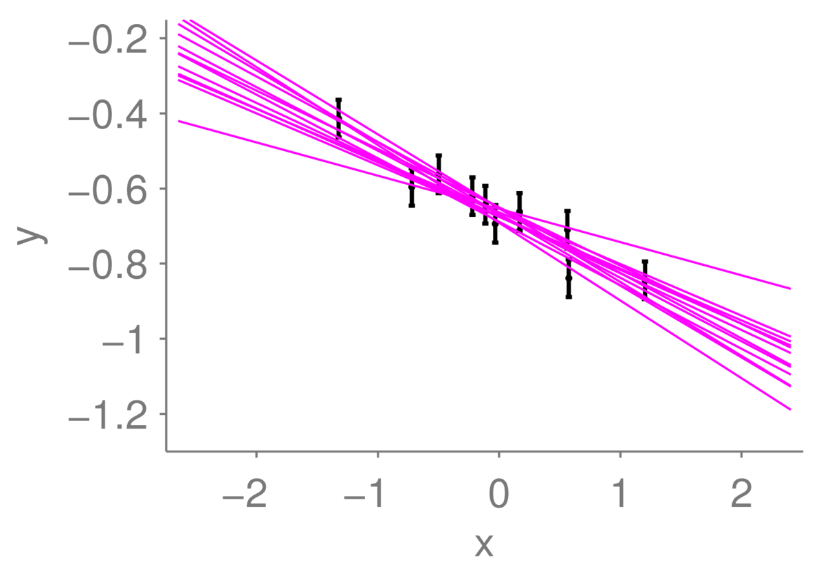
One of the lines does look somewhat less plausible than the others. But it could be close to the true line: maybe the left-most observation happened to have a large amount of noise added to it, and the line is less steep than you think.
If we observe a lot more points, we can be more certain where the underlying line is. The range of plausible lines we might draw should become more limited, perhaps like this:
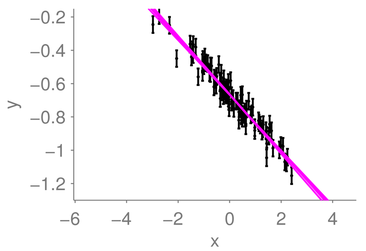
We’ve drawn the lines almost on top of each other, so they appear as one thick line. We can be fairly certain that the true function is somewhere within that tight collection of lines.
If we wanted an intelligent agent to draw these plausible lines of fit for us, how should it do it? Or more generally, how can we systematically express the uncertainty that we should have in conclusions based on limited and noisy data?
One formal approach to handling uncertainty is to use probability distributions to represent our beliefs, and probability theory to update them.4
In the context of line fitting, beliefs are represented by a probability distribution over the parameters. When we are fairly certain, the distribution over parameters should have low variance, concentrating its probability mass on a small region of parameter space. Given only a few datapoints, our distribution over plausible parameters should be much broader.
In the figures above, we drew samples from probability distributions over parameters, and plotted the resulting functions. The lines show just twelve of the many reasonable explanations of the data as represented by a distribution over the model parameters. We got the distributions from Bayes’ rule as described in the next section.
3 Bayes’ rule for beliefs about parameters
To apply probability theory to obtain beliefs we need both a probabilistic model, and prior beliefs about that model.
Our example model for a straight line fit is: \[ f(x;\bw) = w_1x + w_2, \qquad p(y\g x,\bw) = \N(y;\,f(x;\bw),\sigma_y^2). \] So \(w_1\) is the slope parameter and \(w_2\) is the bias parameter, determining the intercept of \(f\). Each \(\bw\) is a point in a 2-dimensional space: the parameter space of \(f\). Each function \(f\) corresponds to a point \(\bw\) in the parameter space and each point \(\bw\) in the parameter space corresponds to a function \(f\). If we knew the parameters \(\bw\), we could compute the function for any \(x\) and simulate what typical observations at that location would look like. However, when learning from data, we don’t know the parameters \(\bw\).
3.1 The prior
Our prior beliefs are represented by a distribution over the parameters, specifying which models we think are plausible before observing any data. For example, if we set: \[ p(\bw) = \N(\bw;\,\mathbf{0},0.4^2\I), \] we think the following functions are all reasonable models we could consider:
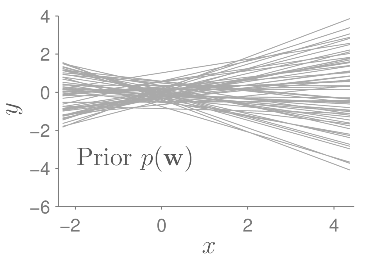
Each of the lines above is a function \(f(x;\bw)\) where we have sampled the parameters \(\bw\) from the prior distribution. They are quite bunched up around the origin. If we wanted to consider larger intercepts at \(x\te0\), we could pick a broader prior on the bias parameter \(w_2\).
3.2 The posterior
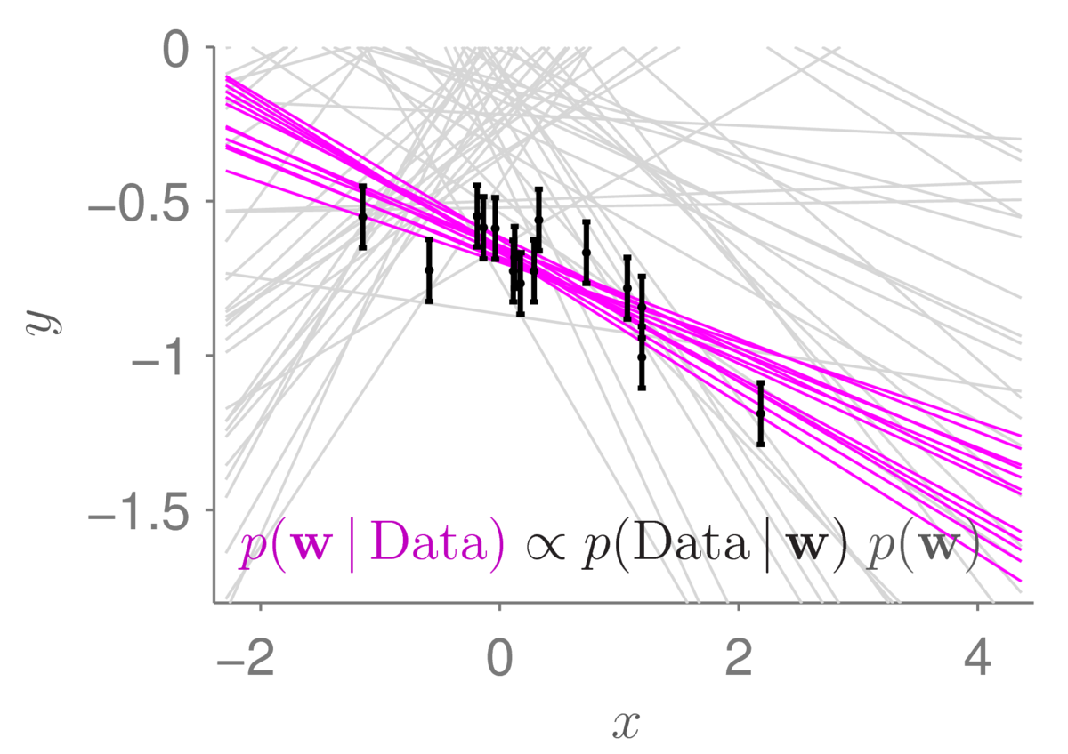
The posterior distribution gives the beliefs about the model parameters that we should have after observing data \(\D\te\{\bx\nth,y\nth\}\). These beliefs are represented by the distribution \(p(\bw\g \D)\), pronounced “p of \(\bw\) given \(\D\)”, and are obtained by Bayes’ rule. For generic data \(\D\) we’d write: \[ p(\bw\g \D) = \frac{p(\D\g\bw)\,p(\bw)}{p(\D)} \propto p(\D\g\bw)\,p(\bw). \] However, for regression we often treat our data as \(\by\te\{y\nth\}\), and condition on the inputs \(X\te\{\bx\nth\}\) as fixed known quantities that don’t affect our prior beliefs. With these assumptions we would instead write: \[ p(\bw\g \D) = p(\bw\g\by, X) = \frac{p(\by\g\bw,X)\,p(\bw)}{p(\by\g X)} \propto p(\by\g\bw, X)\,p(\bw). \] Our posterior belief in the parameters \(\bw\) is proportional to the product of two functions of the parameters, the prior of the parameters \(p(\bw)\), and the likelihood of the parameters \(p(\D\g \bw)\) or \(p(\by\g \bw, X)\). In statistics, likelihood is a technical term for when we consider the probability of the data as a function of parameters (or later model choices).5 The likelihood function is not a probability distribution over the parameters (\(\int p(\D\g \bw)\,\mathrm{d}\bw \ne 1\)).
At a high level, Bayesian inference updates beliefs before seeing the data (given by the prior), so that parameters that are compatible with the data (high likelihood) become more probable under our new beliefs (given by the posterior).
Applying Bayes rule to our toy regression problem (skipping the maths of how to do it for the moment) gives beliefs centred around models that fit the observed data-points. Sampling from that distribution gives the plot below:
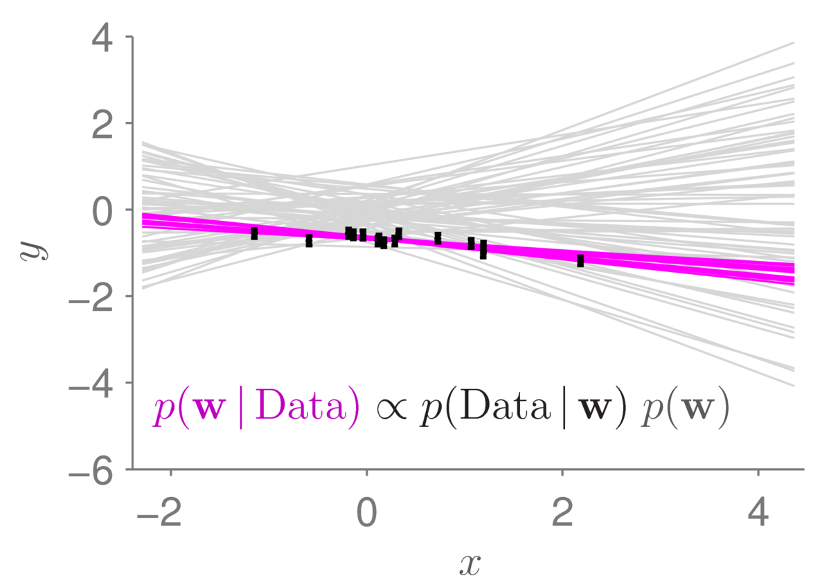
The light gray lines show the samples from the prior distribution that we had before. The small black bars show data points (with error bars). The magenta lines show 12 samples from the posterior distribution. As is usually the case (if our data is useful), the posterior distribution concentrates in a much smaller region of parameter space than the prior. The corresponding straight-line functions are also less spread out. Under the posterior, we only believe that lines passing close to the data are plausible.
Zooming in to the same diagram, we can get a better view of the data and the possible models sampled from the posterior distribution:
The plausible lines sampled from the posterior distribution naturally spread out as we move away from the observed data. The statistical machinery automatically tells us that we are less certain about where the function is as we move away from where we have measured it.
3.3 Computing the Posterior
For general models, the posterior distribution won’t have a convenient form that we can represent with a few parameters. The likelihood is a product of \(N\) terms for \(N\) datapoints, and that product could potentially create a complicated function.
A conjugate prior to a given likelihood is a prior where the product of the prior and likelihood combines to give a distribution with the same functional form as the prior. A Gaussian prior over linear regression weights is conjugate to its linear-Gaussian likelihood, and we obtain a Gaussian posterior: \[\begin{align} p(\bw\g \D) &\propto p(\bw)\,p(\by\g\bw, X),\\ &\propto \N(\bw;\,\mathbf{0},\,\sigma_w^2\mathbb{I})\,\prod_n \N(y\nth;\bw^\top\bphi(\bx\nth),\, \sigma_y^2),\\ &\propto \N(\bw;\,\mathbf{0},\,\sigma_w^2\mathbb{I}) \,\N(\by;\,\Phi\bw,\, \sigma_y^2\I), \end{align}\] where \(\bphi(\bx)\) is an augmented input vector as in earlier notes, for example \(\bphi(x) = [x~~1]^\top\) for fitting a straight line with scalar inputs. As before, \(\Phi\) is a matrix with these augmented vectors in the rows. Here we’ve assumed a zero-mean prior, and a spherical prior covariance. In Murphy’s notation for the prior parameters: \(\bw_0\te\mathbf{0}\) and \(V_0\te\sigma_w^2\mathbb{I}\), which set our beliefs after observing 0 datapoints. We could set the prior mean \(\bw_0\) and covariance \(V_0\) to other values, for example to allow the “bias” parameter that specifies the intercept to vary more.
The posterior is proportional to the exponential of a quadratic in \(\bw\), which means it is a Gaussian distribution. Murphy writes the answer in the form: \(p(\bw\g\D)\te\N(\bw;\,\bw_N, V_N)\), the beliefs after observing \(N\) datapoints. We can identify the posterior mean \(\bw_N\) and covariance \(V_N\) from the linear and quadratic coefficients of \(\bw\) inside the exponential. It’s just linear algebra grunt work, which results in: \[\begin{align} V_N &= \sigma_y^2(\sigma_y^2V_0^{-1} + \Phi^\top \Phi)^{-1}\\ \bw_N &= V_N V_0^{-1}\bw_0 + \frac{1}{\sigma_y^2}V_N \Phi^\top\by. \end{align}\] Or replace \(\Phi\) with \(X\) if you haven’t applied a basis function transformation. We are not expecting you to memorize these expressions!
4 Recommended reading
Bishop Section 1.2.3 introduces the Bayesian interpretation of probabilities. Section 3.3 is on Bayesian linear regression.
Murphy Book 1, Section 4.6 describes the idea behind Bayesian statistics. Chapter 11 introduces linear regression with a probabilistic perspective from the beginning. Bayesian linear regression is in Section 11.7. There is a demo in Figure 11.20 that comes with code.
5 Possible exercises
Set a prior over parameters that lets the intercept of the function vary more, while maintaining the same distribution over slopes as in the demonstration in this note. Plot the straight line functions corresponding to some parameter vectors sampled from your new prior.
If you want to work through the maths and implement a Bayesian inference problem, the following work-up exercise may test if you understand how to go about it. Assume a Gaussian prior over a single number \(m\). Sample a value for \(m\) from this prior and generate \(N\te12\) datapoints from \(\N(m,1)\). What should your posterior be given these observations? You could run a series of trials where you draw a value for \(m\) from the prior, simulate data and compute a posterior. How often is the true value of \(m\) within \(\pm\) one posterior standard deviation of your posterior mean?
6 Further detail
Chapter 3 of David MacKay’s book, describes the undergraduate physics question where he first learned about Bayes’ rule for inferring an unknown parameter. Depending on your background, you may find that story interesting.
Historical note: Using probabilities to describe beliefs has been somewhat controversial over time. There’s no controversy in Bayes’ rule: it’s a rule of probability theory, a direct consequence of the product rule. It’s using Bayes’ rule to obtain beliefs, rather than frequencies, that has been controversial.
Notation: In the following notes we will have variances of multiple quantities, so we need to start labelling them. We use \(\sigma_y^2\) for the conditional variance of an observation \(y\) given the underlying function value \(f\). It is not the variance of the marginal distribution \(p(y)\). We will use this notation again when covering Gaussian processes (GPs). Murphy Book 1 also uses \(\sigma_y^2\) when covering GPs, but plain \(\sigma^2\) for the noise variance for Bayesian linear regression.↩︎
In this note, \(\by\) is an \(N\ttimes1\) vector containing a scalar observation for each training example.↩︎
For example, the Gauss–Markov theorem is another justification, which we won’t discuss.↩︎
For keen students: a justification of this view is outlined in “Probability, frequency and reasonable expectation”, R. T. Cox, American Journal of Physics, 14(1):1–13, 1946. It’s a readable paper.↩︎
You will see some books and papers referring to likelihood of the data, although that goes against traditional usage (cf MacKay, p29). We consider the likelihood of different parameters given the data.↩︎