Week 9 exercises
This is the sixth page of assessed questions, as described in the background notes. These questions form 70% of your mark for Week 9. The introductory questions in the notes and the Week 9 discussion group task form the remaining 30% of your mark for Week 9.
Unlike the questions in the notes, you’ll not immediately see any example answers on this page. However, you can edit and resubmit your answers as many times as you like until the deadline (Friday 20 November 4pm UK time, UTC). This is a hard deadline: This course does not permit extensions and any work submitted after the deadline will receive a mark of zero. See the late work policy.
Queries: Please don’t discuss/query the assessed questions on hypothesis until after the deadline. If you think there is a mistake in a question this week, please email Iain.
Please only answer what’s asked. Markers will reward succinct to-the-point answers. You can put any other observations in the “Add any extra notes” button (but this is for your record, or to point out things that seemed strange, not to get extra credit). Some questions ask for discussion, and so are open-ended, and probably have no perfect answer. For these, stay within the stated word limits, and limit the amount of time you spend on them (they are a small part of your final mark).
Feedback: We’ll return feedback on your submission via email by Friday 27 November.
Good Scholarly Practice: Please remember the University requirements for all assessed work for credit. Furthermore, you are required to take reasonable measures to protect your assessed work from unauthorised access. For example, if you put any such work on a public repository then you must set access permissions appropriately (permitting access only to yourself). You may not publish your solutions after the deadline either.
1 Nearest neighbours and learning parameters
The \(K\)-nearest-neighbour (KNN) classifier predicts the label of a feature vector by finding the \(K\) nearest feature vectors in the training set. The label predicted is the label shared by the majority of the training neighbours. For binary classification we normally choose \(K\) to be an odd number so ties aren’t possible.
KNN is an example of a non-parametric method, which means that no fixed-size vector of parameters (like \(\bw\) in logistic regression) summarizes the training data. Instead, the complexity of the function represented by the classifier grows with the number of training examples \(N\). Often, the whole training set needs to be stored so that it can be consulted at test time. (Gaussian processes are also a non-parametric method.)
Non-parametric methods can have parameters. We could modify the KNN classifier by taking a linear transformation of the data \(\bz = A\bx\), and finding the \(K\) nearest neighbours using the new \(\bz\) features. We’d like to learn the matrix \(A\), but for \(K\te1\), the training error is 0 for all \(A\) (the nearest neighbour of a training point is itself, which has the correct label by definition).
A loss function that could evaluate possible transformations \(A\) is the leave-one-out (LOO) classification error, defined as the fraction of errors made on the training set when the \(K\) nearest neighbours for a training item don’t include the point being classified itself.
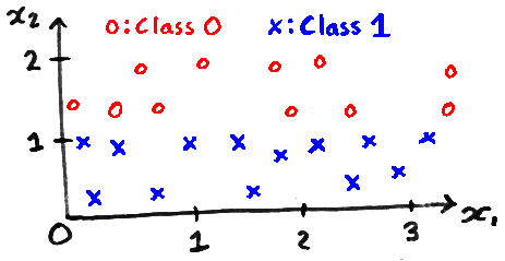
The identity transformation, which does nothing, is: \[A = \left[\begin{array}{cc} 1 & 0\\ 0 & 1\\ \end{array}\right]. \] Write down a matrix \(A\) where the 1-nearest neighbour classifier has lower LOO error than using the identity matrix for the data below. Explain why it works in two or three sentences. [15 marks]
You can right-click on the equation above to get the TeX code, which you can then modify for your answer for \(A\).
Explain why we can’t minimize the LOO error with respect to the matrix \(A\) using gradient-based optimization. Write no more than 100 words. [15 marks]
2 A neural network for the CT data
This question continues from last week’s exercise, predicting the location in the body that a CT scan slice comes from.
The data (26 MB) is unchanged. You don’t need to download it again.
The support code has been expanded, please use: w9_support.py
Your code must be entirely written by you, except for using NumPy and the support code (and the SciPy import that it makes). Please don’t duplicate the support code in your answers to a) and b), just include an import line.
In Question 1b last week you already fitted a small neural network. The logistic regression classifiers are sigmoidal hidden units, and a linear output unit predicts the outputs. However, you didn’t fit the parameters jointly to minimize a single cost function.
A regularized square cost function and gradients for this neural network are implemented in the nn_cost function provided this week. Please read this code. You can use the nn_cost function (as you used cost functions last week) to optimize all of the parameters at once.
Include code that fits the neural network with a sensible random initialization of the parameters and regularizer
alpha=10, and that prints the root-mean-square error on the training set. Include an example number that you obtain at the end of your answer. We should be able to run your code as provided, assuming the data and support code are in the current directory. [10 marks]Include code that again fits the neural network with
alpha=10, but that initializes the parameters to the values fitted by last week’s procedure. Your code should print the root-mean-square error on the training set. Again include an example number that you obtain at the end of your answer. Please make your code stand-alone so that it can run as-is (duplicate anything required from last week and/or part a). [10 marks]Is one initialization strategy better than the other? Is fitting the neural network jointly (as in part a or b) better than first fitting classifiers and then a regression model (as you did last week)? Justify your answers clearly.
Your answer to this part should be standalone: include any numbers that you are using in your argument, even if you’ve quoted them before in previous parts or last week. Another student should be able to understand where your numbers came from. However, don’t include any code in this part. Write no more than 150 words. [20 marks]