Bayesian logistic regression
So far we have only performed probabilistic inference in two particularly tractable situations: 1) small discrete models: inferring the class in a generative classifier, the card game, the robust logistic regression model. 2) “linear-Gaussian models”, where the observations are linear combinations of variables with Gaussian beliefs, to which we add Gaussian noise.
For most models, we cannot compute the equations for making Bayesian predictions exactly. Logistic regression will be our working example. We’ll look at how Bayesian predictions differ from regularized maximum likelihood. Then we’ll look at different ways to approximately compute the integrals.
1 Logistic regression
As a quick review, the logistic regression model gives the probability of a binary label given a feature vector: \[ P(y\te1\g\bx, \bw) \,=\, \sigma(\bw^\top\bx) \,=\, 1/(1+e^{-\bw^\top\bx}). \] We usually add a bias parameter \(b\) to the model, making the probability \(\sigma(\bw^\top\bx\tp b)\). Although the bias is often dropped from the presentation, to reduce clutter. We can always work out how to add a bias back in, by including a constant element in the input features \(\bx\).
You’ll see various notations used for the training data \(\D\). The model gives the probability of a vector of outcomes \(\by\) associated with a matrix of inputs \(X\) (where the \(n\)th row is \(\bx^{(n)\top}\)). Maximum likelihood fitting maximizes the probability: \[ P(\by\g X, \bw) = \prod_n \sigma(z\nth \bw^\top\bx\nth), \qquad \text{where}~z\nth = 2y\nth \tm 1,~~\text{if}~~ y\nth \in \{0,1\}. \] For compactness, we’ll write this likelihood as \(P(\D\g\bw)\), even though really only the outputs \(\by\) in the data are modelled. The inputs \(X\) are assumed fixed and known.
Logistic regression is most frequently fitted by a regularized form of maximum likelihood. For example L2 regularization fits an estimate \[ \bw^* = \argmax_\bw \left[\log P(\by\g X, \bw) - \lambda \bw^\top\bw\right]. \] We find a setting of the weights that make the training data appear probable, but discourage fitting extreme settings of the weights, that don’t seem reasonable. Usually the bias weight will be omitted from the regularization term.
Just as with simple linear regression, we can instead follow a Bayesian approach. The weights are unknown, so predictions are made considering all possible settings, weighted by how plausible they are given the training data.
2 Bayesian logistic regression
The posterior distribution over the weights is given by Bayes’ rule: \[ p(\bw\g\D) = \frac{P(\D\g\bw)\,p(\bw)}{P(\D)} \propto P(\D\g\bw)\,p(\bw). \] The normalizing constant is the integral required to make the posterior distribution integrate to one: \[ P(\D) = \int P(\D\g\bw)\,p(\bw)\intd\bw. \]
The figures below1 are for five different plausible sets of parameters, sampled from the posterior \(p(\bw\g\D)\).2 Each figure shows the decision boundary \(\sigma(\bw^\top\bx)\te0.5\) for one parameter vector as a solid line, and two other contours given by \(\bw^\top\bx\te\pm1\).

The axes in the figures above are the two input features \(x_1\) and \(x_2\). The model included a bias parameter, and the model parameters were sampled from the posterior distribution given data from the two classes as illustrated. The arrow, perpendicular to the decision boundary, illustrates the direction and magnitude of the weight vector.
Assuming that the data are well-modelled by logistic regression, it’s clear that we don’t know what the correct parameters are. That is, we don’t know what parameters we would fit after seeing substantially more data. The predictions given the different plausible weight vectors differ substantially.
The Bayesian way to proceed is to use probability theory to derive an expression for the prediction we want to make: \[\begin{align} P(y\g \bx, \D) &= \int p(y,\bw\g \bx, \D)\intd\bw\\ &= \int P(y\g \bx,\bw)\,p(\bw\g\D)\intd\bw. \end{align}\] That is, we should average the predictive distributions \(P(y\g\bx,\bw)\) for different parameters, weighted by how plausible those parameters are, \(p(\bw\g\D)\). Contours of this predictive distribution, \(P(y\te1\g\bx,\D) \in \{0.5, 0.27, 0.73, 0.12,0.88\}\), are illustrated in the left panel below. Predictions at some constant distance away from the decision boundary are less certain when further away from the training inputs. That’s because the different predictors above disagreed in regions far from the data.

Again, the axes are the input features \(x_1\) and \(x_2\). The right hand figure shows \(P(y\te1\g \bx,\bw^*)\) for some fitted weights \(\bw^*\). No matter how these fitted weights are chosen, the contours have to be linear. The parallel contours mean that the uncertainty of predictions falls at the same rate when moving away from the decision boundary, no matter how far we are from the training inputs.
It’s common to describe L2 regularized logistic regression as MAP (Maximum a posteriori) estimation with a Gaussian \(\N(\mathbf{0},\sigma_w^2\eye)\) prior on the weights. The “most probable”3 weights, coincide with an L2 regularized estimate: \[ \bw^* = \argmax_\bw \left[\log p(\bw\g \D)\right] = \argmax_\bw \left[ \log P(\D\g \bw) - \frac{1}{2\sigma_w^2}\bw^\top\bw \right]. \] MAP estimation is not a “Bayesian” procedure. The rules of probability theory don’t tell us to fix an unknown parameter vector to an estimate. We could view MAP as an approximation to the Bayesian procedure, but the figure above illustrates that it is a crude one: the Bayesian predictions (left) are qualitatively different to the MAP ones (right).
Unfortunately, we can’t evaluate the integral for predictions \(P(y\g\bx,\D)\) in closed form. Making model choices for Bayesian logistic regression is also computationally challenging. The marginal probability of the data, \(P(\D)\), is the marginal likelihood of the model, which we might write as \(P(\D\g\M)\) when we are evaluating some model choices \(\M\) (such as basis functions and hyperparameters). We also can’t evaluate the integral for \(P(\D)\) in closed form.
3 The logistic regression posterior is sometimes approximately Gaussian
We’re able to do some integrals involving Gaussian distributions. The posterior distribution over the weights \(p(\bw\g\D)\) is not Gaussian, but we can make progress if we can approximate it with a Gaussian.
Below is an example to illustrate how the posterior over the weights can look non-Gaussian. We have a Gaussian prior with one sigmoidal likelihood term. Here we assume we know the bias4 is 10, and we have one datapoint with \(y\te1\) at \(x\te-20\): \[ \begin{align} p(w) \,&\propto\, \N(w; 0, 1)\\ p(w\g \D) \,&\propto\, \N(w; 0, 1)\,\sigma(10 - 20w). \end{align} \] We are now fairly sure that the weight isn’t a large positive value, because otherwise we’d have probably seen \(y\te0\). We (softly) slice off the positive region5 and renormalize to get the posterior distribution illustrated below:
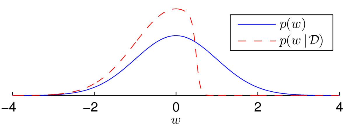
The distribution is asymmetric and so clearly not Gaussian. Every time we multiply the posterior by a sigmoidal likelihood, we softly carve away half of the weight space in some direction. While the posterior distribution has no neat analytical form, the distribution over plausible weights often does look Gaussian after many observations.
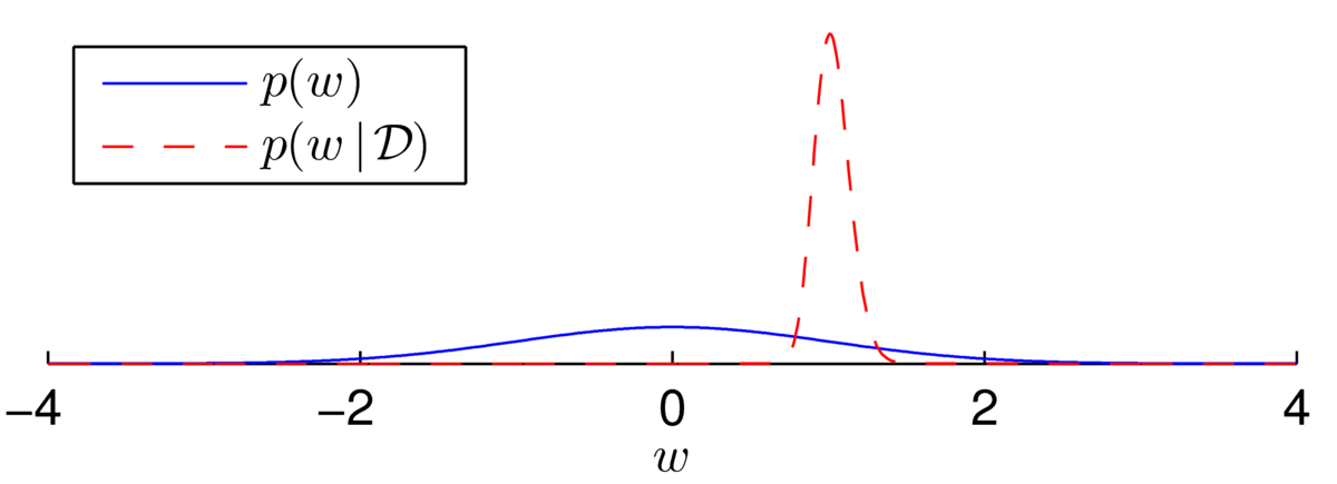
As another example, let’s consider \(N\te500\) labels, \(\{z\nth\}\), generated from a logistic regression model with no bias and with \(w\te1\) at \(x^{(n)}\sim \N(0,10^2)\). Then, \[ \begin{align} p(w) \,&\propto\, \N(w; 0, 1)\\ p(w\g \D) \,&\propto\, \N(w; 0, 1)\,\prod_{n=1}^{500}\sigma(wx^{(n)}z^{(n)}), \qquad z\nth \in \{\pm1\}. \end{align} \] The posterior now appears to be a beautiful bell-shape:
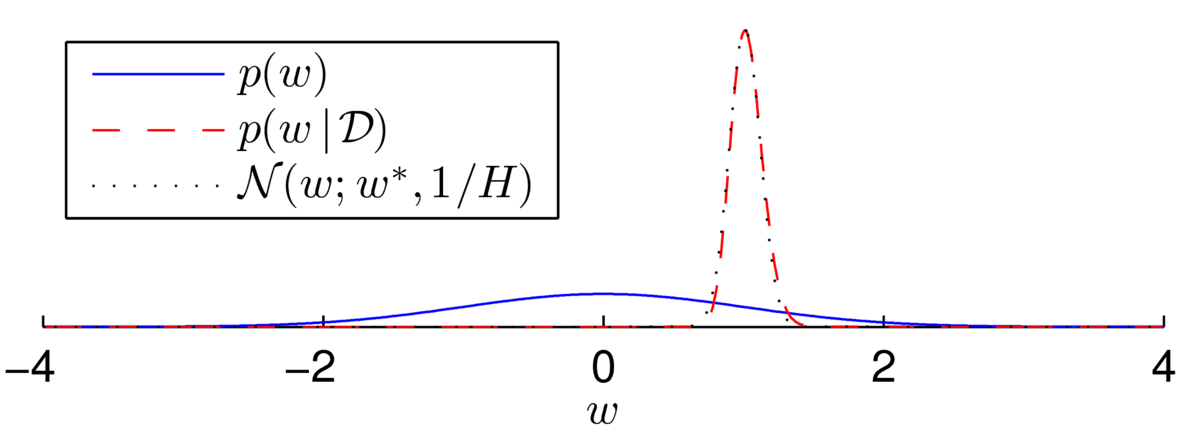
Fitting a Gaussian distribution (using the Laplace approximation, next note) shows that the distribution isn’t quite Gaussian… but it’s close:
The two figures in this section are extracts from Figure 41.7 of MacKay’s textbook (p499).↩︎
It’s not obvious how to generate samples from \(p(\bw\g\D)\), and in fact it’s hard to do exactly. These samples were drawn approximately with a “Markov chain Monte Carlo” method.↩︎
“Most probable” is problematic for real-valued parameters. Really we are picking the weights with the highest probability density. But those weights aren’t well-defined, because if we consider a non-linear reparameterization of the weights, the maximum of the pdf will be in a different place. That’s why we prefer to describe estimating the weights as “regularized maximum likelihood” or “penalized maximum likelihood” rather than MAP.↩︎
Perhaps we have many datapoints and have fitted the bias precisely, but we have one datapoint that has a novel feature turned on, and the example is showing the posterior over the weight that interacts with that one feature.↩︎
If it’s not obvious what’s going on, plot \(\sigma(10-20w)\) against \(w\). We are multiplying our prior by this soft step function, which multiplies the prior by nearly one on the left, and nearly zero on the right.↩︎