The Laplace approximation applied to Bayesian logistic regression

There are multiple ways that we could try to fit a distribution with a Gaussian form. For example, we could try to match the mean and variance of the distribution. The Laplace approximation is another possible way to approximate a distribution with a Gaussian. It can be seen as an incremental improvement of the MAP approximation to Bayesian inference, and only requires some additional derivative computations.

In Bayesian logistic regression, we can only evaluate the posterior distribution up to a constant: we can evaluate the joint probability \(p(\bw,\D)\), but not the normalizer \(P(\D)\). We match the shape of the posterior using \(p(\bw,\D)\), and then the approximation can be used to approximate \(P(\D)\).

The Laplace approximation sets the mode of the Gaussian approximation to the mode of the posterior distribution, and matches the curvature of the log probability density at that location. We need to be able to evaluate first and second derivatives of \(\log P(\bw,\D)\).

The rest of the note just fills in the details. We’re not adding much to MacKay’s textbook pp341–342, or Murphy’s book Sections 4.6.8.2 and 10.5.1. Although we try to go slightly more slowly and show some pictures of what can go wrong.

1 Matching the distributions

First of all we find the most probable setting of the parameters: \[ \bw^* = \argmax_\bw\, p(\bw\g\D) = \argmax_\bw\, \log p(\bw,\D). \] The conditional probability on the left is what we intuitively want to optimize. The maximization on the right gives the same answer, but contains the term we will actually compute. Reminder: why do we take the log?¹

We usually find the mode of the distribution by minimizing an ‘energy’, which is the negative log-probability of the distribution up to a constant. For a posterior distribution, we can define the energy as: \[ E(\bw) = - \log p(\bw,\D), \qquad \bw^* = \argmin_\bw E(\bw). \] We minimize it as usual, using a gradient-based numerical optimizer.

The minimum of the energy is a turning point. For a scalar variable \(w\) the first derivative \(\pdd{E}{w}\) is zero and the second derivative gives the curvature of this turning point: \[ H = \left. \frac{\partial^2 E(w)}{\partial w^2} \right|_{w=w^*}. \] The notation means that we evaluate the second derivative at the optimum, \(w=w^*\). If \(H\) is large, the slope (the first derivative) changes rapidly from a steep descent to a steep ascent. We should approximate the distribution with a narrow Gaussian. Generalizing to multiple variables \(\bw\), we know \(\nabla_\bw E\) is zero at the optimum and we evaluate the Hessian, a matrix with elements: \[ H_{ij} = \left. \frac{\partial^2 E(\bw)}{\partial w_i\partial w_j} \right|_{\bw=\bw^*}. \] This matrix tells us how sharply the distribution is peaked in different directions.

For comparison, we can find the optimum and curvature that we would get if our distribution were Gaussian. For a one-dimensional distribution, \(\N(\mu, \sigma^2)\), the energy (the negative log-probability up to a constant) is: \[ E_\N(w) = \frac{(w-\mu)^2}{2\sigma^2}. \] The minimum is \(w^*=\mu\), and the second derivative \(H = 1/\sigma^2\), implying the variance is \(\sigma^2 = 1/H\). Generalizing to higher dimensions, for a Gaussian \(\N(\bmu,\Sigma)\), the energy is: \[ E_\N(\bw) = \frac{1}{2} (\bw-\bmu)^\top \Sigma^{-1} (\bw-\bmu), \] with \(\bw^*=\bmu\) and \(H = \Sigma^{-1}\), implying the covariance is \(\Sigma = H^{-1}\).

Therefore matching the minimum and curvature of the ‘energy’ (negative log-probability) to those of a Gaussian energy gives the Laplace approximation to the posterior distribution: \[ \fbox{$\displaystyle p(\bw\g\D) \approx \N(\bw;\, \bw^*, H^{-1}) $} \]

2 Approximating the normalizer \(Z\)

Evaluating our approximation for a \(D\)-dimensional distribution gives: \[ p(\bw\g\D) = \frac{p(\bw,\D)}{P(\D)} \approx \N(\bw;\, \bw^*, H^{-1}) = \frac{|H|^{1/2}}{(2\pi)^{D/2}} \exp\left( -\frac{1}{2} (\bw-\bw^*)^\top H(\bw-\bw^*)\right). \] At the mode \(\bw^*\te\bw\), the exponential term disappears and we get: \[ \frac{p(\bw^*,\D)}{P(\D)} \approx \frac{|H|^{1/2}}{(2\pi)^{D/2}}, \qquad \fbox{$\displaystyle P(\D) \approx \frac{p(\bw^*,\D) (2\pi)^{D/2}}{|H|^{1/2}}$}. \] An equivalent expression is \[\fbox{$P(\D) \approx p(\bw^*,\D)\, |2\pi H^{-1}|^{1/2},$}\] where \(|\cdot|\) means take the determinant of the matrix.

When some people say “the Laplace approximation”, they are referring to this approximation of the normalization \(P(\D)\), rather than the intermediate Gaussian approximation to the distribution.

3 Computing logistic regression predictions

Now we return to the question of how to make Bayesian predictions (all implicitly conditioned on a set of model choices \(\M\)): \[\begin{align} P(y\g \bx, \D) &= \int p(y,\bw\g \bx, \D)\intd\bw\\ &= \int P(y\g \bx,\bw)\,p(\bw\g\D)\intd\bw. \end{align}\]

We can approximate the posterior with a Gaussian, \(p(\bw\g\D)\approx \N(\bw;\,\bw^*, H^{-1})\), using the Laplace approximation (or variational methods, next week). Using this approximation, we still have an integral with no closed form solution: \[\begin{align} P(y\te1\g \bx, \D) &\approx \int \sigma(\bw^\top\bx)\,\N(\bw;\,\bw^*, H^{-1})\intd\bw\\ &= \E_{\N(\bw;\,\bw^*, H^{-1})}\!\left[ \sigma(\bw^\top\bx)\right]. \end{align}\] However, this expectation can be simplified. Only the inner product \(a\te\bw^\top\bx\) matters, so we can take the average over this scalar quantity instead. The linear combination \(a\) is a linear combination of Gaussian beliefs, so our beliefs about it are also Gaussian. By now you should be able to show that \[ p(a) = \N(a;\; {\bw^*}^\top\bx,\; \bx^\top H^{-1}\bx). \] Therefore, the predictions given the approximate posterior, are given by a one-dimensional integral: \[\begin{align} P(y\te1\g \bx, \D) &\approx \E_{\N(a;\;{\bw^*}^\top\bx,\; \bx^\top H^{-1}\bx)}\left[ \sigma(a)\right]\\ &= \int \sigma(a)\,\N(a;\;{\bw^*}^\top\bx,\; \bx^\top H^{-1}\bx)\intd{a}. \end{align}\] One-dimensional integrals can be computed numerically to high precision.

Bishop p. 220 and Murphy Section 10.5.2.2 review a further approximation, also called probit approximation, which is quicker to evaluate and provides an interpretable closed-form expression: \[ P(y\te1\g \bx, \D) \approx \sigma(\kappa\, {\bw^*}^\top\bx), \qquad \kappa = \frac{1}{\sqrt{1+\frac{\pi}{8}\bx^\top H^{-1}\bx}}. \] Under this approximation, the predictions use the most probable or MAP weights. However, the activation is scaled down (with \(\kappa\)) when the activation is uncertain, so that predictions will be less confident far from the data (as they should be).

4 Is the Laplace approximation reasonable?

If we think that the Energy is well-behaved and sharply peaked around the mode of the distribution, we might think that we can approximate it with a Taylor series. In one dimension we write \[ \begin{align} E(w^* + \delta) &\approx E(w^*) \;+\; \left.\pdd{E}{w}\right|_{w^*}\delta \;+\; \frac{1}{2}\left.\frac{\partial^2 E}{\partial w^2}\right|_{w^*}\delta^2\\ &\approx E(w^*) \;+\; \frac{1}{2}H\delta^2, \end{align} \] where the second term disappears because \(\pdd{E}{w}\) is zero at the optimum. In multiple dimensions this Taylor approximation generalizes to: \[ E(\bw^* + \bdelta) \approx E(\bw^*) + {\textstyle\frac{1}{2}}\bdelta^\top \!H\bdelta. \] A quadratic energy (negative log-probability) implies a Gaussian distribution. The distribution is close to the Gaussian fit when the Taylor series is accurate.

For models with a fixed number of identifiable parameters, the posterior becomes tightly peaked in the limit of large datasets. Then the Taylor expansion of the log-posterior doesn’t need to be extrapolated far and will be accurate. Search term for more information: “Bayesian central limit theorem”.

5 The Laplace approximation doesn’t always work well!

Despite the theory above, it is easy for the Laplace approximation to go wrong.

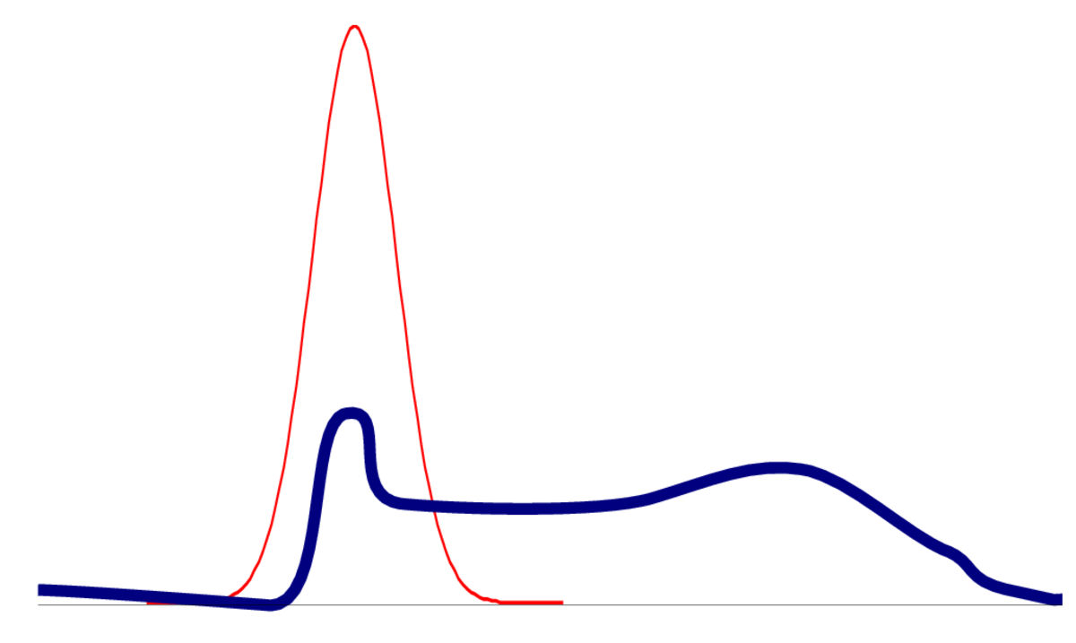
In high dimensions, there are many directions in parameter space where there might only be a small number of informative datapoints. Then the posterior could look like the first asymmetrical example in this note.

If the mode and curvature are matched, but the distribution is otherwise non-Gaussian, then the value of the densities won’t match².

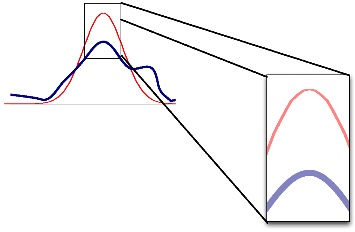
As a result, the approximation of \(P(\D)\) will be poor.

One way for a distribution to be non-Gaussian is to be multi-modal. The posterior of logistic regression only has one mode, but the posterior for neural networks will be multimodal. Even if capturing one mode is reasonable, an optimizer could get stuck in bad local optima.

In models with many parameters, the posterior will often be flat in some direction, where parameters trade off each other to give similar predictions. When there is zero curvature in some direction, the Hessian isn’t positive definite and we can’t get a meaningful approximation.

6 Further Reading

Bishop covers the Laplace approximation and application to Bayesian logistic regression in Sections 4.4 and 4.5.

Murphy touches the Laplace approximation in Sections 4.6.8.2 and 10.5.1.

Similar material is covered by MacKay, Ch. 41, pp492–503, and Ch. 27, pp341–342.

The Laplace approximation was used in some of the earliest Bayesian neural networks although — as presented here — it’s now rarely used. However, the idea does occur in recent work, such as on uncertainty units for Laplace-approximated networks (Kristiadi et al., UAI, 2021) and on continual learning (Kirkpatrick et al., Google Deepmind, 2017) and a more sophisticated variant is used by the popular statistical package, R-INLA.